
Backtracking
The Idea
Think of a solution as a sequence of decisions: include this element or not, put a queen in this column, use this digit. The set of all partial solutions forms a tree. The root is "nothing decided yet", each edge is one decision, and each leaf is a complete candidate. Backtracking walks this tree depth-first, and it abandons a branch as soon as it can tell that no complete solution lies below it.
The Template
Nearly every backtracking function has the same shape. Learn it once and write it from memory:
func explore(state) {
	if state is a complete solution {
		record a COPY of it
		return
	}
	for each choice available now {
		if the choice is not allowed {
			continue // PRUNE early
		}
		choose it           // change the state
		explore(new state)
		un-choose it        // restore the state exactly
	}
}
The demo 55_backtracking_template.go applies this template to subsets, permutations, combinations, and parentheses. The three lines choose, explore, un-choose are the heart of the method. The recursion itself is the same divide-and-conquer stack you saw in Recursion; backtracking adds the undo step.
What Must Be Undone
Whatever choose changes, un-choose must change back. A partial solution may live in several places: a path slice, a "used" array, a visited mark in a grid, a set of taken columns. If you update three things when you choose, you restore three things when you undo. Forgetting one is the most common backtracking bug, and it produces results that look plausible but are wrong: extra solutions, missing solutions, or a search that quietly stops working after the first branch.
List, Count, or Optimize?
| The question | Technique |
|---|---|
| List every solution, or find one that meets many constraints | backtracking |
| Count solutions, or find the best value, and subproblems repeat | dynamic programming |
| The best value, and a provable local rule exists | greedy |
| The best value, no repeating subproblems, but good bounds exist | branch and bound (below) |
The lesson repeats one check: when a problem can be solved both ways, the demos compare the two. The lists produced by backtracking have the same size as the count from the DP, and a walk through a grid is checked against a bitmask table.
Listing All Solutions
The first five problems all list their answers. Each shows one new idea. All are in 55_backtracking_template.go.
Subsets
For each element there are two choices: leave it out or put it in. A leaf appears after every element has been decided, so a set of n elements has 2n subsets.
func subsets(nums []int) [][]int {
	var result [][]int
	var path []int
	var explore func(i int)
	explore = func(i int) {
		if i == len(nums) {
			result = append(result, slices.Clone(path)) // a COPY: path changes later
			return
		}
		explore(i + 1) // choice 1: leave nums[i] out
		path = append(path, nums[i])
		explore(i + 1)            // choice 2: put nums[i] in
		path = path[:len(path)-1] // un-choose: remove it again
	}
	explore(0)
	return result
}
Record a Copy
path is one slice that keeps changing during the search. Storing path itself stores a slice header that shares the same backing array, so later changes rewrite the stored answers. The demo runs the same code without slices.Clone and prints:
correct:  [[] [3] [2] [2 3] [1] [1 3] [1 2] [1 2 3]]
no copy:  [[] [1] [1] [1 2] [1] [1 2] [1 2] [1 2 3]]
The second list has eight entries, but the wrong ones. Always copy when you record. For a string built from a byte slice, string(path) already copies.
Permutations
At each position, choose any element that is not used yet. Now there are two things to restore: the path and the used flag.
for i := range nums {
	if used[i] {
		continue // already in the path: prune
	}
	used[i] = true // choose
	path = append(path, nums[i])
	explore()
	path = path[:len(path)-1] // un-choose: BOTH changes must be undone
	used[i] = false
}
There are n! results: 6 for three elements, 5,040 for seven. The demo checks that each n from 0 to 7 gives n! distinct lists, each using every number once.
Inputs with Duplicates
For {1, 2, 2} the plain algorithms produce eight subsets, because the two 2s are treated as different elements. Sort the input first. Then at each level of the tree, skip a value equal to the one just tried at the same level: choosing the same value in the same position again only repeats a branch.
for i := start; i < len(nums); i++ {
	if i > start && nums[i] == nums[i-1] {
		continue // same value already tried at this level
	}
	// choose, explore, un-choose as usual
}
The result is [] [1] [1 2] [1 2 2] [2] [2 2]. Note the condition i > start: skipping is only correct for a value that was already tried at this level, not for the first element after descending. For permutations the rule is different: use an equal value only after its equal predecessor is in the path (!used[i-1] means skip), which forces equal values to appear in their sorted order. The demo compares both with "enumerate everything and remove duplicates" on 400 random inputs with many repeats.
Combination Sum and Pruning
Find every way to reach a target by adding numbers from a list, using each number any number of times. Combinations, not sequences: {2, 3} and {3, 2} are the same, so the next choice may never go back to an earlier candidate. The loop starts at index from, and passes i (not i + 1) to allow repeats.
![Search tree for combination sum with candidates 2, 3 and 5 and target 5. The solutions [2,3] and [5] are green, [2,2] is a dead end, and the branches [2,5], [3,3], [3,5] and [2,2,...] are pruned because the next number exceeds what is still needed](/roadmap/dsa/img/dsa-backtracking-tree.svg)
The search tree for candidates {2, 3, 5} and target 5. Two branches succeed, one dead-ends, and four are never visited.
for i := from; i < len(cands); i++ {
	if prune && cands[i] > remaining {
		break // sorted: every later candidate is even larger
	}
	path = append(path, cands[i])
	explore(i, remaining-cands[i]) // i, not i+1: a number may repeat
	path = path[:len(path)-1]
}
Pruning is what separates backtracking from brute force. With the candidates sorted, once one number is larger than what is still needed, every later number is too, so the loop stops. The set of solutions is identical; only the number of visited states changes: over 500 random problems the demo visits 24,603 states without the check and 14,723 with it. The number of lists also matches the DP count from Dynamic Programming, so the DP acts as an independent check.
Balanced Parentheses
Build a string of n opening and n closing brackets from left to right. Two rules prune the tree so that only valid strings are ever built: add ( only while fewer than n have been used, and add ) only while it closes something (close < open). The number of results follows the Catalan numbers: 1 1 2 5 14 42 132 429 1430 4862 16796 for n = 0 to 10. For n up to 6 the demo compares the result with all 22n bracket strings filtered by a validity check. Here the constraint is not tested at the end but built into the choices, which is the best kind of pruning: there are no dead ends at all.
Pruning and Choice Order
Two questions decide whether a search finishes in a millisecond or in a year. Pruning: how early can you detect a dead end? Choice order: which decision do you make next? Both are shown on two classic puzzles in 56_queens_sudoku.go.
N-Queens
Place n queens on an n × n board so that no two share a row, a column, or a diagonal. Forcing one queen per row removes the row constraint entirely: the search decides only the column of each row's queen. A queen at (r, c) attacks along three lines, and each line has a simple number: the column c, the diagonal r − c, and the anti-diagonal r + c. Two queens share a line exactly when they share one of these numbers, so three sets of taken values are the whole state.
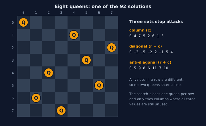
One of the 92 solutions for n = 8. The three lists of numbers on the right are all distinct: that is what "no two queens attack" means.
for c := 0; c < n; c++ {
	d, a := r-c+n-1, r+c
	if usedCol[c] || usedDiag[d] || usedAnti[a] {
		continue // attacked: prune before going deeper
	}
	nodes++
	col[r] = c
	usedCol[c], usedDiag[d], usedAnti[a] = true, true, true // choose
	place(r + 1)
	usedCol[c], usedDiag[d], usedAnti[a] = false, false, false // un-choose
}
Three things are chosen and three are undone. The demo prints the count and the number of tried placements for each n and checks them against the known solution table and against all column permutations for n ≤ 8:
| n | 4 | 5 | 6 | 7 | 8 | 9 | 10 |
|---|---|---|---|---|---|---|---|
| solutions | 2 | 10 | 4 | 40 | 92 | 352 | 724 |
| placements tried | 16 | 53 | 152 | 551 | 2,056 | 8,393 | 35,538 |
For n = 8 there are 4,426,165,368 ways to put eight queens on 64 squares. The pruned search tries 2,056 placements.
Sets as Bit Masks
The three sets can live in three integers. A set bit means "taken", and the diagonal masks shift by one bit per row, because a diagonal moves one column sideways for every row down:
free := all &^ (cols | diag | anti)
for free != 0 {
	bit := free & -free // lowest free column
	free &^= bit
	count += place(cols|bit, (diag|bit)<<1&all, (anti|bit)>>1)
}
One &^ finds all legal columns of a row at once, and there are no arrays to restore: the masks are passed by value, so un-choosing is free. For n = 13 (73,712 solutions) the array version takes about 300 ms and the bitmask version about 40 ms on the test machine. The same idea as the bitmask state in Dynamic Programming, used here with recursion instead of a table.
Sudoku
Fill a 9 × 9 grid so every row, column, and 3 × 3 box holds the digits 1 to 9. The state is three arrays of nine bit sets (row, column, box). The candidates for an empty cell are the digits missing from all three:
func (s *solver) candidates(r, c int) uint16 {
	return ^(s.rows[r] | s.cols[c] | s.box[r/3*3+c/3]) & 0x3FE // bits 1..9
}
Choosing puts the digit into all three sets; un-choosing clears it from all three. After a solution is found, the demo checks every answer against the rules and against the given digits.
Fail First: the Most Constrained Cell
Which empty cell should be filled next? The simple answer is "the first one in reading order". A much better answer is the cell with the fewest candidates. A cell with one candidate is forced, and a cell with zero candidates proves at once that the current branch is a dead end. Failing early is cheaper than discovering the same dead end after filling a dozen other cells. This is the "minimum remaining values" heuristic, and the results are dramatic:
| Puzzle | first empty cell | most constrained cell |
|---|---|---|
| a newspaper puzzle | 4,209 states | 52 states |
| a puzzle built to defeat brute force | gave up after 5,000,000 states | solved in 58,234 states |
The choice order does not change which solutions exist, only how much of the tree is explored to reach them. For the same reason it pays to decide the most constrained thing first in any search: the queen row with the fewest safe columns, the graph vertex with the most neighbours.
Grids and Strings
Grids and strings bring new kinds of state to undo: a visited mark in the grid, a prefix of letters, an end position for the next piece. Demo with five problems, each compared with an independent method: 57_search_and_paths.go.
Word Search
Is a word spelled by a path of adjacent cells (up, down, left, right) that never reuses a cell? The visited mark is the state: set it when you choose a cell and clear it when you undo. Writing the mark into the grid itself (a # that matches no letter) needs no extra array:
saved := g[r][c]
g[r][c] = '#' // choose: this cell is now used
for _, d := range dirs {
	if dfs(r+d[0], c+d[1], k+1) {
		g[r][c] = saved // leave the grid as we found it, even on success
		return true
	}
}
g[r][c] = saved // un-choose
return false
The line g[r][c] = saved after the loop is easy to forget. Without it, every failed branch leaves a wall of # behind and later searches see a broken grid. The demo compares the result with an oracle that lists every path in the grid and looks the word up in the list, on 1,500 random grids.
Many Words: Prune by Prefix
To find every word from a dictionary in a grid, following every path up to the longest word is wasteful. Keep the set of all prefixes of the dictionary words, and stop the moment the letters so far start no word:
cur += string(grid[r][c])
nodes++
if prune && !prefix[cur] {
	return // no dictionary word starts with cur: abandon the branch
}
On the small board in the demo, 400 states shrink to 72. Over 300 random boards the search drops from 91,149 states to 15,743, and the found words match the "list every path and filter" oracle every time. A trie stores the prefixes far more compactly, which is the subject of Advanced Trees.
Letter Combinations and Palindrome Partitions
Two more problems have a simple choice at each step. Letter combinations of a phone number chooses one letter for each digit, so the number of results is the product of the letter counts (the demo checks this on random digit strings). Palindrome partitions lists every way to cut a string into palindromes. The choice is where the next piece ends, and only palindromic pieces are tried, so bad cuts never grow. "aaba" has three partitions: a|a|b|a, a|aba, and aa|b|a. The demo compares 500 random strings with all 2n−1 ways of cutting them. Contrast this with the palindrome DP in Dynamic Programming, which only counts the fewest cuts and lists nothing.
Walking Every Cell
Given a grid with a start cell, an end cell, and walls, count the routes from start to end that visit every free cell exactly once. The state to undo is the visited mark. There are two prunings: never step on a used cell, and reaching the end before every cell is visited is a dead end.
visited[nr][nc] = true // choose
dfs(nr, nc, left-1)
visited[nr][nc] = false // un-choose
On a 3 × 4 grid there are 4 such routes, found in 195 states. To check the count without trusting the same method, the demo builds the bitmask DP from Dynamic Programming (ways[mask][cell]) and compares both on 400 random grids with walls. Two completely different algorithms agreeing is strong evidence that both are right. The DP is faster on large grids, but it needs 2cells memory; backtracking with good pruning can handle cases the table cannot hold.
Optimization: Branch and Bound
To find the best solution, plain backtracking still visits every solution. Branch and bound adds one idea: at each state, compute an optimistic bound, the best value this branch could possibly reach, and abandon the branch when even that cannot beat the best solution found so far. Demo with two problems: 58_branch_and_bound.go.
What Makes a Good Bound
- It must be optimistic. It may never be lower than the true best of the branch, or a branch that contains the best solution gets cut. This is the one rule that must not be broken.
- A tighter bound prunes more, but costs more to compute in every state. The best bounds come from a relaxed version of the problem that is easy to solve.
- Find a good solution early. The bound can only prune against a solution that already exists, so try the promising choice first.
Graph Colouring and Symmetry
Colour the vertices of a graph with the fewest colours so that neighbours differ. Try 1 colour, then 2, then 3, until a colouring exists. The prune is the constraint itself: skip a colour that a neighbour already has. The new idea is symmetry breaking. Colours are interchangeable: swapping "red" and "blue" everywhere gives another valid colouring, and a search that ignores this repeats every failed branch once for each permutation of the colours. So a vertex may reuse a colour that is already in use, or open the next new colour, but never a colour that skips ahead:
limit := m // colours 0..m-1 are allowed
if symmetry {
	limit = min(m, used+1) // reuse a colour, or open just the next new one
}
for c := 0; c < limit; c++ {
The demo runs three variants on five well-known graphs (the chromatic numbers are 5, 3, 2, 3, and 4):
| Graph | Colours | plain | + symmetry | + symmetry, high degree first |
|---|---|---|---|---|
| K5 (complete) | 5 | 94 | 20 | 20 |
| cycle C5 | 3 | 17 | 13 | 13 |
| cycle C6 | 2 | 9 | 9 | 9 |
| Petersen graph | 3 | 22 | 18 | 18 |
| Grötzsch graph | 4 | 495 | 99 | 103 |
The gap grows with the graph. On 20 random graphs of 14 vertices the total number of states is 140,718 for the plain search, 6,591 with symmetry breaking, and 828 with symmetry breaking and high-degree vertices first: a 170-fold reduction from two small ideas. The demo also checks the colour count against a brute force that tries every possible colouring, on 300 random graphs of up to 7 vertices.
Knapsack with a Bound
For the 0/1 knapsack, the bound comes from the problem's own relaxation: the fractional knapsack from Greedy Algorithms. If the remaining items could be cut, greedy by value per weight is optimal, so its value is an upper bound on what the whole branch can reach. Real answers cannot do better, because items cannot really be cut.
bound := func(i, room, value int) float64 {
	total := float64(value)
	for ; i < n && room > 0; i++ {
		if sorted[i].w <= room {
			room -= sorted[i].w
			total += float64(sorted[i].v)
		} else {
			total += float64(sorted[i].v) * float64(room) / float64(sorted[i].w)
			break
		}
	}
	return total
}
The search sorts the items by value per weight, tries "take it" before "leave it", and returns from any state whose bound (rounded down, since real values are whole numbers) does not exceed the best value found so far. The demo compares three modes on 300 random instances against the DP table from Dynamic Programming:
| Mode | States visited (300 instances) |
|---|---|
| plain: try every subset | 1,294,664 |
| skip items that no longer fit | 408,129 |
| also prune by the fractional bound | 4,655 |
The real payoff is where the DP cannot go. With weights up to 108 and a capacity of over a billion, the DP table would need 50 billion cells for 45 items. The bounded search solves the instance in 109 states. The demo checks the method against every subset for 22-item instances of the same size, where 222 subsets is still feasible. The two techniques complement each other: use the DP when the numbers are small, and the bound when the numbers are large but the structure is friendly. Branch and bound has no guarantee, though: a badly chosen bound or an unlucky instance can still explore an exponential number of states.
Designing a Backtracking Search
A Checklist
- Decision. What is decided at each level: an element (include or not), a position (which value), a cell (which digit)?
- State. What must be stored so the next level can tell which choices are legal (path, used flags, taken columns, visited marks)?
- Goal. When is the state a complete solution, and what is recorded (a copy)?
- Constraint. Which choices are illegal? Test them before choosing, not after the branch is complete.
- Undo. List every change made by choosing, and reverse each one.
- Order and bound. Which decision comes first, and which choice is tried first? Is there a cheap optimistic bound?
Estimating the Size of the Tree
Before you run a search, estimate its worst case from the shape of the tree. A yes/no decision per element gives 2n leaves. Choosing an order of n items gives n!. Choosing one of k values at each of n positions gives kn. Backtracking is practical up to roughly n = 20 to 25 for 2n and n = 10 to 12 for n! without pruning, and much further when the constraints prune well, as in the queens and Sudoku above. If the pruned tree is still too large, look for a different technique: a DP if subproblems repeat, or a heuristic if a good answer is enough.
When Backtracking Is Not Enough
Real constraint-solving tools build on this lesson. SAT solvers add "learn from a dead end" so the same conflict is not met again, constraint solvers propagate each choice through the remaining variables before searching, and metaheuristics such as simulated annealing give up exactness to search vast spaces. The template, the undo step, and the habit of failing early carry over to all of them.
Common Pitfalls
Backtracking bugs rarely crash. They produce lists with a wrong item, a missing item, or a search that is silently too slow.
Storing the Path Instead of a Copy
The recorded solutions all change when path changes, as the demo's aliasing output shows. Clone at the moment of recording.
Forgetting to Undo One Change
If choosing changes a slice, a flag, and a counter, un-choosing must restore all three. Put the choose and un-choose lines next to each other and read them as a pair. A symptom is a search that works on the first branch and then finds too few solutions.
Pruning Too Late, or Wrongly
Testing a constraint only at the leaf turns backtracking into brute force. Test it before choosing. Conversely, a prune that is too aggressive, such as a bound that is not optimistic, silently discards valid solutions: the search finishes fast and returns a wrong answer, which is why every demo has an oracle.
Duplicates and Ordering
With repeated values or interchangeable choices, the same solution is found many times. Sort and skip repeated values at the same level, or break symmetry as in the colouring above. Test with inputs full of repeats; random inputs with distinct values hide this bug.
Recursion Depth and Shared State
The recursion depth equals the number of decisions, which is small for most puzzles but can be large for a walk through a big grid. Go grows the stack dynamically, so deep recursion is rarely fatal, but each level costs memory. Avoid package-level variables for search state: a closure over local variables, as the demos use, keeps searches independent and makes the undo easier to reason about.
Practice Lab
For each exercise, write down the decision, the state, and the constraint before any code, then decide what the recursion must undo.
Run the Demos
- In 55_backtracking_template.go, delete the line
used[i] = falseinpermutations. How many checks fail, and which results are missing? - In 56_queens_sudoku.go, change the un-choose line in
queensso thatusedDiag[d]is never cleared. How many of the ten board sizes now give a wrong count, and why do the smallest sizes survive? - In 57_search_and_paths.go, delete the line
g[r][c] = saved // un-chooseafter the loop inwordExists. What happens to later words on the same grid? - In 58_branch_and_bound.go, replace the fractional term in
boundbytotal += 0. The bound is no longer optimistic. Which checks fail, and why does the search still finish quickly?
Exercises
- Subsets with a target. List every subset of a set of positive numbers that adds up to a target. Add the pruning "stop when the sum exceeds the target", then a stronger prune using the sum of the numbers that remain. Count the states each version visits.
- Restore IP addresses. Cut a string of digits into four numbers from 0 to 255 with no leading zeros. What is the decision at each level, and how small is the tree?
- Knight's tour. Move a knight so that it visits every square of a small board exactly once. Try neighbour squares in order of fewest onward moves (Warnsdorff's rule) and compare the number of states with plain order.
- Sudoku with a second heuristic. Add "hidden singles" to the solver in demo 56: if a digit fits in only one cell of a row, column or box, place it. How much does it reduce the states on the hard puzzle?
- Count with both methods. Count the ways to place n non-attacking rooks on an n × n board with some cells forbidden. Solve it by backtracking, then with a bitmask DP over columns, and compare the results and the running times.
Continue with Advanced Trees, where the tree becomes the data structure instead of the search space.