
Complexity Analysis
Why Analyze Cost
Two correct solutions can differ by hours of run time on the same input. You need a way to compare them that does not depend on which laptop you own, which compiler version you use, or how busy the machine is at the moment.
Counting Steps, Not Seconds
Seconds depend on hardware; the number of basic steps does not. A basic step is any operation whose cost does not depend on the input size: an arithmetic operation, a comparison, reading nums[i], assigning a variable. We count how many such steps an algorithm performs as a function of the input size, and ignore how long each individual step takes.
What "n" Means
n is the size of the input measured in the unit that drives the work: the number of elements in a slice, the number of characters in a string, the number of vertices in a graph. When there are several independent sizes, give each its own letter — a graph has V vertices and E edges, a text of length n is searched for a pattern of length m.
Big O Notation
Big O describes the upper bound of the growth rate. It answers "at most how fast does the cost grow?" and deliberately throws away details that do not change the answer for large inputs.
Definition
A cost function f(n) is O(g(n)) if there exist constants c > 0 and n₀ such that f(n) ≤ c · g(n) for every n ≥ n₀. In words: beyond some input size, f never grows faster than a constant multiple of g. For example, f(n) = 3n + 5 is O(n), because 3n + 5 ≤ 4n whenever n ≥ 5 (c = 4, n₀ = 5).
Drop Constants and Lower Terms
Two simplification rules follow from the definition:
- Constant factors disappear: 5n and n/2 are both O(n). Constants depend on hardware and implementation; growth does not.
- Only the dominant term remains: n² + 100n + 7 is O(n²). For n = 10,000 the n² term contributes 100,000,000 steps, the 100n term only 1,000,000.
This is why an O(n) algorithm with a large constant eventually beats an O(n²) algorithm with a tiny one — "eventually" being the n₀ in the definition.
Big Omega and Big Theta
Big O is an upper bound, and two related notations complete the picture:
| Notation | Meaning | Example |
|---|---|---|
| O(g) | grows at most like g | Linear search is O(n) |
| Ω(g) | grows at least like g | Any comparison sort is Ω(n log n) in the worst case |
| Θ(g) | grows exactly like g (both bounds) | Summing a slice is Θ(n) |
In everyday engineering "O" is used loosely to mean the tight bound. When precision matters — proving a lower bound, for example — use Ω and Θ.
Best, Worst, and Average Case
The same algorithm can cost different amounts on inputs of the same size. Linear search finds the target at index 0 in one step (best case) but scans all n elements when it is absent (worst case). Unless stated otherwise, a complexity refers to the worst case, because it is a guarantee. The average case needs an assumption about input distribution; hash maps are the standard example — O(1) on average, O(n) in the worst case when all keys collide.
Common Complexity Classes
A handful of growth rates cover almost every algorithm you will meet. The chart shows how quickly they separate: by n = 20, the exponential curve has left the chart while the logarithmic one has barely moved.
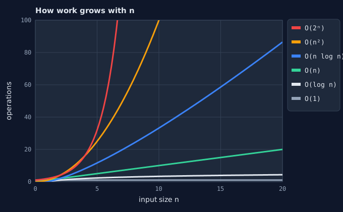
Growth of the common classes for n from 0 to 20. The vertical axis is capped at 100 operations; O(2ⁿ) crosses it just before n = 7 and O(n²) reaches it at n = 10.
Growth Table
The table turns the chart into numbers. Assuming roughly 10⁸ simple operations per second (a rough figure for compiled code on modern hardware), it shows which classes remain practical as n grows.
| Class | Name | n = 10 | n = 1,000 | n = 1,000,000 | Typical example |
|---|---|---|---|---|---|
| O(1) | constant | 1 | 1 | 1 | index a slice, map lookup (avg) |
| O(log n) | logarithmic | 3 | 10 | 20 | binary search |
| O(n) | linear | 10 | 1,000 | 10⁶ | scan a slice |
| O(n log n) | linearithmic | 33 | ~10⁴ | ~2·10⁷ | merge sort, slices.Sort |
| O(n²) | quadratic | 100 | 10⁶ | 10¹² (hours) | compare all pairs |
| O(2ⁿ) | exponential | 1,024 | ~10³⁰¹ | impossible | try every subset |
Run 03_growth_rates.go to see these counts produced by real loops.
Reading Complexity from Code
Most of the time you can read the complexity directly from the shape of the loops. Three rules cover the common cases: sequential blocks add, nested loops multiply, and a loop that halves its range runs log n times.
// Sequential blocks ADD: O(n) + O(n) = O(2n) = O(n)
for i := 0; i < n; i++ { /* O(1) work */ }
for i := 0; i < n; i++ { /* O(1) work */ }

// Nested loops MULTIPLY: O(n) * O(n) = O(n^2)
for i := 0; i < n; i++ {
	for j := 0; j < n; j++ { /* O(1) work */ }
}

// Triangular nesting is still O(n^2): 0+1+...+(n-1) = n(n-1)/2
for i := 0; i < n; i++ {
	for j := 0; j < i; j++ { /* O(1) work */ }
}

// Halving the range each step: log2(n) iterations -> O(log n)
for size := n; size > 1; size /= 2 { /* O(1) work */ }

// Hidden loops count too: slices.Contains scans the slice,
// so this "single" loop is really O(n * m)
for _, x := range queries {       // m iterations
	if slices.Contains(data, x) { // O(n) each
		hits++
	}
}
Multiple Inputs
When a function receives two independent inputs, keep both sizes in the result. Iterating over a and then over b is O(n + m); iterating over b for every element of a is O(n · m). Writing O(n²) for the second case would be wrong when one input is much smaller than the other — searching a 10-character pattern in a 1 GB log is very different from comparing two 1 GB files.
Space Complexity
Memory is a cost too, and it often decides between two algorithms with the same time complexity. The Two Sum map version is faster than the brute-force version precisely because it spends O(n) memory.
Auxiliary Space
Auxiliary space is the extra memory an algorithm allocates beyond its input. Finding a maximum needs O(1) auxiliary space (one variable); detecting duplicates with a map needs O(n); building an n × n distance table needs O(n²). When people say "in-place", they mean O(1) auxiliary space.
Recursion Uses Stack Space
Every active recursive call holds a stack frame, so recursion depth counts as space. A recursive sum over n elements uses O(n) stack space even though it allocates nothing explicitly. The Recursion lesson shows the call stack in detail.
Amortized Cost
Some operations are usually cheap but occasionally expensive. Amortized analysis averages the cost over a long sequence of operations, giving a guarantee for the whole sequence even when individual operations vary.
Slice append
A Go slice has a fixed capacity. When append finds it full, the runtime allocates a larger backing array and copies every element — an O(n) step. Because capacity grows by a factor (about 2× for small slices, tapering toward 1.25× for large ones), these expensive copies become rarer as the slice grows.
With pure doubling, appending n elements triggers copies of 1, 2, 4, …, n/2 elements, and that geometric series sums to less than n. Total work for n appends is therefore under 2n, so each append costs O(1) amortized. Any constant growth factor above 1 gives the same result; growing by a fixed amount (say +10 each time) would not, and would make n appends O(n²).
// Pre-sizing avoids the repeated copies entirely when n is known.
out := make([]int, 0, n) // len 0, capacity n: one allocation
for i := 0; i < n; i++ {
	out = append(out, i*i) // never reallocates
}
Measuring in Go
Analysis predicts; measurement confirms. Use both: an analysis without measurement can miss a hidden cost, and a measurement without analysis cannot be extrapolated to larger inputs.
Doubling Experiment
Run the code on n, 2n, 4n, … and compute the ratio between consecutive times. A ratio near 2 indicates linear growth, near 4 quadratic, near 8 cubic. The ratio cancels out the machine's speed, which is exactly the property Big O relies on. Once you know the growth law you can predict the cost of inputs too large to test.
Full experiment comparing an O(n²) and an O(n) duplicate detector, with a prediction for n = 4,000,000: 04_doubling_experiment.go.
Benchmarks with testing.B
For precise measurements, Go's testing package runs a function enough times to get a stable result and reports nanoseconds per operation. Put benchmarks in a _test.go file and run go test -bench=..
// dup_test.go — run with: go test -bench=. -benchmem
package main

import (
	"fmt"
	"testing"
)

func BenchmarkHasDupSet(b *testing.B) {
	for _, n := range []int{1_000, 10_000, 100_000} {
		input := distinct(n) // setup is outside the timed loop
		// sub-benchmarks report one line per input size
		b.Run(fmt.Sprint(n), func(b *testing.B) {
			// b.Loop (Go 1.24+) repeats the body until timing is stable;
			// on older versions use: for i := 0; i < b.N; i++
			for b.Loop() {
				hasDupSet(input)
			}
		})
	}
}
The -benchmem flag adds allocations per operation, which makes space costs visible too.
From Constraints to Target Complexity
Problem constraints tell you which complexity is required before you design anything. Using the rough budget of 10⁸ simple operations per second:
| Input size n | Acceptable complexity | Typical technique |
|---|---|---|
| ≤ 20 | O(2ⁿ), O(n!) | backtracking, brute-force subsets |
| ≤ 500 | O(n³) | triple loops, Floyd–Warshall |
| ≤ 5,000 | O(n²) | all pairs, simple DP tables |
| ≤ 10⁶ | O(n log n) | sorting, heaps, divide and conquer |
| ≤ 10⁸ | O(n) | single pass, hashing, two pointers |
| larger | O(log n), O(1) | binary search, math formula |
Common Pitfalls
Complexity errors rarely come from misapplying the definition; they come from costs that are not visible in the code.
Hidden Loops
Library calls have their own complexity. slices.Contains, strings.Index, and slices.Insert are all O(n). Building a string with s += part inside a loop copies the whole string each time — O(n²) in total — because Go strings are immutable. Use strings.Builder, whose appends are amortized O(1).
Constants Still Matter
Big O describes growth, not speed at a particular size. For small inputs an O(n²) insertion sort often beats O(n log n) algorithms because it has tiny constants and good cache behavior — which is why Go's own sort switches to insertion sort for short sub-slices. Measure when n is small and the code is hot.
Average Is Not a Guarantee
Map operations are O(1) on average, not in the worst case. Go randomizes its hash seed per map, which protects against inputs crafted to collide, but a real-time system with hard deadlines should still reason about worst cases, and prefer structures with guaranteed bounds (balanced trees, sorted slices) where they matter.
Practice Lab
Build the reflex of estimating cost before running code, then checking the estimate.
Run the Demos
- Run 03_growth_rates.go. Add an O(n³) column (three nested loops) and predict its value at n = 64 before running.
- Run 04_doubling_experiment.go on your machine. Your absolute times will differ from anyone else's; check whether the ratios match.
Exercises
- Give the complexity of: a loop from 1 to n where the counter doubles (
i *= 2) and the body loops from 0 to i. Hint: sum the geometric series. - Rewrite a loop that builds a comma-separated string with
+=to usestrings.Builder, and use a doubling experiment to show the change from quadratic to linear. - A problem states n ≤ 200,000. Which of O(n²), O(n log n), and O(n) are acceptable? Explain with the operations budget.
Next lesson: Recursion & the Call Stack.