Graph Traversal

Graph Vocabulary and Representations

A graph has V vertices and E edges. Edges can be directed (a follows b, a imports b) or undirected (a road, a friendship), and can carry a weight (distance, cost, latency). The degree of a vertex is its number of edges. A graph is sparse when E is close to V and dense when E approaches V². Almost all real graphs are sparse. Demo with all three representations: 37_graph_representations.go.

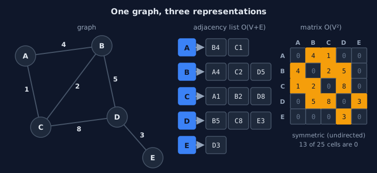
The same five-vertex graph three ways. The matrix spends a cell on every pair, including the 13 pairs with no edge.

Choosing a Representation

For a sparse graph with a million vertices and four million edges, a matrix of booleans would need about 1,000 GB, while adjacency lists need about 200 MB. Use adjacency lists by default.

Adjacency Lists in Go

Number the vertices 0 to V − 1 and store a slice of outgoing edges per vertex. If vertices have names or IDs, map them to indices once, at the boundary, with a map[string]int. The algorithms can then use fast slices instead of maps.

type Edge struct {
	From, To, Weight int
}

// Graph is an adjacency list: adj[u] holds the edges leaving u.
type Graph struct {
	adj      [][]Edge
	directed bool
}

func (g *Graph) AddEdge(u, v, w int) {
	g.adj[u] = append(g.adj[u], Edge{u, v, w})
	if !g.directed {
		g.adj[v] = append(g.adj[v], Edge{v, u, w}) // store both directions
	}
}

Implicit Graphs

Many graphs are never stored at all. In a maze, image, or game map, the neighbours of cell (r, c) are computed when needed: the up to four adjacent cells that are inside the grid and not walls. Word ladders, puzzle states, and configuration spaces work the same way. The traversal algorithms do not change; only the "get neighbours" step does.

Breadth-First Search

BFS explores in waves: first the start vertex, then everything one edge away, then two edges away, and so on. A FIFO queue produces exactly this order. Because each wave is completed before the next begins, the first time BFS reaches a vertex, it has found a path with the fewest edges. Demo with path reconstruction, a maze, multi-source BFS, and an oracle check on random graphs: 38_bfs.go.

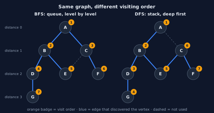
BFS (left) visits by distance. DFS (right) follows one branch to the end before backtracking. The blue edges form each search's tree.

The Algorithm

func bfs(adj [][]int, start int) (dist, parent []int) {
	n := len(adj)
	dist = make([]int, n)
	parent = make([]int, n)
	for i := range dist {
		dist[i], parent[i] = -1, -1 // -1 doubles as "not visited yet"
	}
	dist[start] = 0
	queue := []int{start}
	for head := 0; head < len(queue); head++ { // index instead of popping: O(1)
		u := queue[head]
		for _, v := range adj[u] {
			if dist[v] == -1 { // mark when ENQUEUED, not when dequeued,
				dist[v] = dist[u] + 1 // or a vertex can enter the queue twice
				parent[v] = u
				queue = append(queue, v)
			}
		}
	}
	return dist, parent
}

Each vertex is enqueued at most once and each edge is examined once from each end, so BFS runs in O(V + E) time and O(V) memory. Reading the queue by index is a simple alternative to the ring buffer from Stacks & Queues, because BFS never needs the slots again.

Reconstructing the Path

parent[v] records which vertex discovered v. The parent links form a BFS tree of shortest paths from the start. To get the path to a target, follow parents back to the start and reverse:

func pathTo(parent []int, target int) []int {
	var path []int
	for v := target; v != -1; v = parent[v] {
		path = append(path, v)
	}
	slices.Reverse(path)
	return path
}

Grids and Multiple Sources

On a grid, the same loop finds the shortest route through a maze. The demo solves a 5 × 10 maze and draws the path. With multi-source BFS, all sources start in the queue at distance 0, and the result is each vertex's distance to its nearest source, such as every house to the closest hospital, in a single O(V + E) pass rather than one BFS per source.

Depth-First Search

DFS follows one path as deep as possible, then backtracks to the most recent vertex that still has unexplored edges. Recursion provides that last-in, first-out order automatically; an explicit stack does the same without risking a stack overflow on huge graphs. DFS does not find shortest paths, but the order in which it enters and leaves vertices reveals the graph's structure. Demo: 39_dfs.go.

Recursive and Iterative DFS

func dfsOrder(adj [][]int, start int) []int {
	visited := make([]bool, len(adj))
	var order []int
	var visit func(u int)
	visit = func(u int) {
		visited[u] = true
		order = append(order, u)
		for _, v := range adj[u] {
			if !visited[v] {
				visit(v) // go deeper before trying u's next neighbour
			}
		}
	}
	visit(start)
	return order
}

The iterative version pops a vertex from a stack, skips it if it is already visited, and pushes its neighbours in reverse order so they come off the stack in the same order as in the recursive version. The demo checks on random graphs that both versions produce identical orders.

Connected Components

In an undirected graph, one DFS (or BFS) visits exactly one connected component. Loop over all vertices and start a new search from each vertex that is not yet visited. The number of searches is the number of components. Flood fill in paint programs and counting islands on a map work the same way on grids.

Detecting Cycles with Three Colours

In a directed graph, a cycle exists exactly when DFS finds an edge back to a vertex that is still on the current path. Three colours track this: white (not visited), gray (on the current path), and black (finished). An edge to a black vertex is harmless; it leads into a part of the graph that was fully explored and has no path back.

func hasCycleDirected(adj [][]int) bool {
	const white, gray, black = 0, 1, 2
	color := make([]int, len(adj))
	var visit func(u int) bool
	visit = func(u int) bool {
		color[u] = gray
		for _, v := range adj[u] {
			if color[v] == gray || (color[v] == white && visit(v)) {
				return true
			}
		}
		color[u] = black
		return false
	}
	for u := range adj {
		if color[u] == white && visit(u) {
			return true
		}
	}
	return false
}

Two-Colouring: Bipartite Graphs

A graph is bipartite if its vertices can be split into two groups with every edge crossing between them: workers and jobs, students and courses. Colour the start vertex, give each neighbour the opposite colour, and report failure if an edge joins two vertices of the same colour. That happens exactly when the graph contains an odd cycle.

Topological Sort

A topological order lists every vertex before all the vertices it points to: a package before the packages that import it, a course before the courses that require it. It exists if and only if the directed graph has no cycle, which makes it a DAG (directed acyclic graph). Demo with both algorithms, cycle detection, and a critical-path schedule: 40_topological_sort.go.

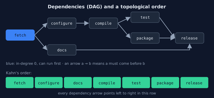
In a topological order, every dependency arrow points from left to right.

Kahn's Algorithm

Count each vertex's incoming edges (its in-degree). Vertices with in-degree 0 have no remaining prerequisites and can go first. Output one, remove its outgoing edges by decrementing its neighbours' in-degrees, and repeat. If some vertices are never output, they lie on a cycle.

for len(ready) > 0 {
	u := ready[0]
	ready = ready[1:]
	order = append(order, u)
	for _, v := range adj[u] {
		indeg[v]-- // u is done: one fewer prerequisite for v
		if indeg[v] == 0 {
			ready = append(ready, v)
		}
	}
}
// Vertices on a cycle never reach in-degree 0 and are never emitted.
return order, len(order) == len(adj)

DFS Postorder

In a DAG, a vertex finishes (turns black) only after every vertex it points to has finished. Appending each vertex when it finishes and reversing the list therefore gives a topological order. The gray check from cycle detection comes for free.

Scheduling: the Critical Path

A topological order lets you process vertices so that all inputs of a vertex are final before the vertex itself. This is dynamic programming on a DAG, which Phase 4 develops in depth. With task durations, the earliest finish time of each task is its duration plus the latest finish among its prerequisites. The longest chain of dependencies, the critical path, is the minimum time for the whole project, however many workers you add.

Union-Find

BFS and DFS answer connectivity questions for a fixed graph. When edges keep arriving and you must answer "are x and y connected?" after each one, re-running a traversal every time costs O(V + E) per question. A disjoint-set union (DSU, or union-find) answers each question in nearly constant time. Demo with a relabelling oracle and a worst-case comparison: 41_union_find.go.

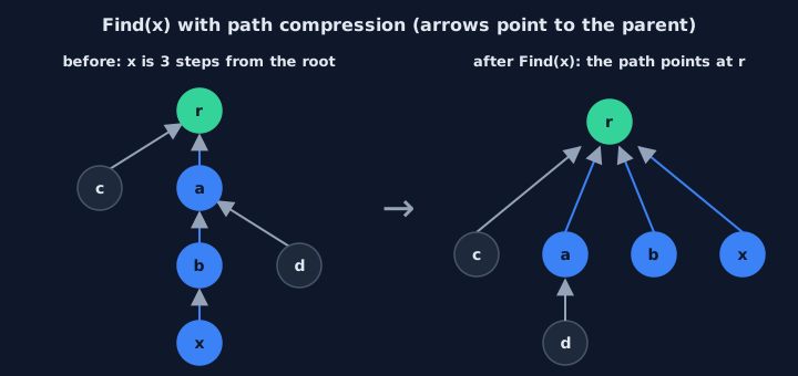
Path compression: after one Find(x), every node on the path points directly to the root.

Find and Union

Each group is stored as a tree of parent pointers, and the root is the group's representative. Find follows parents to the root; Union attaches one root under the other. Union returns false when both elements are already in the same group. For an edge, that means adding it would close a cycle, which is exactly what Kruskal's algorithm in the next lesson needs.

func (d *DSU) Find(x int) int {
	root := x
	for d.parent[root] != root {
		root = d.parent[root]
	}
	for d.parent[x] != root { // second pass: repoint every node to the root
		next := d.parent[x]
		d.parent[x] = root
		x = next
	}
	return root
}

func (d *DSU) Union(x, y int) bool {
	rx, ry := d.Find(x), d.Find(y)
	if rx == ry {
		return false
	}
	if d.size[rx] < d.size[ry] {
		rx, ry = ry, rx // make rx the larger tree
	}
	d.parent[ry] = rx
	d.size[rx] += d.size[ry]
	d.groups--
	return true
}

Why It Is Almost Constant Time

Without care, unions can build a long chain, and each Find costs O(n). In the demo, 16,384 finds on such a chain take 134 million parent steps. Two tricks fix this. Union by size hangs the smaller tree under the larger, so a node's depth increases only when its tree at least doubles in size, which limits the height to log₂ n (the demo's worst case reaches exactly 14 for n = 2¹⁴). Path compression then flattens every path that Find walks. Together they give an amortized cost of O(α(n)) per operation, where α, the inverse Ackermann function, is at most 4 for any realistic n.

Common Pitfalls

Graph bugs usually come from bookkeeping: visited marks, edge directions, and recursion depth.

Marking Visited Too Late

If BFS marks a vertex when it is dequeued instead of when it is enqueued, the same vertex can enter the queue many times. On dense graphs the queue grows to O(E) and the running time multiplies. Mark it at the moment you add it to the queue.

Forgetting the Reverse Edge

An undirected edge must be stored in both adjacency lists. Missing the reverse edge turns the graph into a directed one: BFS then misses vertices, and component counts come out wrong.

Deep Recursion

Go's goroutine stacks grow dynamically, so recursive DFS on a path of a million vertices does not crash immediately as it would in C, but each frame costs memory and time, and the maximum stack size is 1 GB by default. For very large graphs, use the iterative version with an explicit stack.

Practice Lab

For each exercise, first name the vertices and the edges. Then choose BFS, DFS, topological sort, or union-find.

Run the Demos

1. In 38_bfs.go, turn the queue into a stack: take u from the end of the slice instead of the front. The oracle check fails. Why do the distances become wrong even though every vertex is still visited?
2. In 39_dfs.go, treat black like gray in hasCycleDirected (color[v] != white). Which of the two small example graphs now reports a false cycle?
3. In 40_topological_sort.go, move order = append(order, u) in dfsTopo to just after color[u] = gray, so vertices are recorded when they are entered instead of when they finish. The DFS order stops being valid: find an edge that it violates.
4. In 41_union_find.go, remove the second loop of Find (path compression). How deep does the tree stay after one Find per element?

Exercises

1. Word ladder. Find the shortest chain from "cold" to "warm" that changes one letter at a time, where each word must be in a dictionary. What are the vertices and edges, and do you need to build the graph explicitly?
2. Course schedule. Given prerequisites as pairs, return a valid course order or report the courses that lie on a cycle.
3. Accounts merge. Each account lists email addresses; accounts that share an address belong to the same person. Group them with union-find.
4. Rotting oranges. In a grid, rotten oranges infect adjacent fresh ones every minute. Compute when the last orange rots using multi-source BFS.

Next: Shortest Paths & MST, which adds weights to edges.