GPU & Distributed Computing

This lesson starts with the distributed model: how workers are created, how work and code reach them, and how the per-process memory boundary changes the way you write code. It then moves to the GPU — why its model is fundamentally different, how array programming carries over, and when a custom kernel is worth writing. The final chapters cover the pitfalls of scale-out and how to decide whether you need any of this at all.

The Distributed Model

Julia's Distributed standard library starts processes and gives you a small vocabulary for talking to them: addprocs, remotecall, @spawnat, and @everywhere. The model is deliberately concrete: what you create is a process, not a magic pool.

Adding Workers

Workers are created at start-up with -p or later with addprocs. On one machine they behave like extra processes; on a cluster the same call goes through a cluster manager.

# Start with workers:  julia -p 4      (or add them later)
using Distributed

nprocs()                              # 1 without workers
addprocs(4)                           # spawn four local worker processes
nprocs()                              # 5 — the master plus four workers

workers()                             # [2, 3, 4, 5] — the worker ids
myid()                                # 1 — the master process id

# Every process has its own memory: a variable here does not exist there
x = 42
remotecall_fetch(() -> isdefined(Main, :x), 2)     # false

# Worker processes are full Julia processes: they load their own packages
# and pay their own compilation costs.

# Stop them when the work is finished
rmprocs(2:5)
nprocs()                              # 1

# On a cluster the same API goes through a manager
#   using Distributed, SlurmClusterManager
#   addprocs(SlurmManager(); partition = "compute", ntasks = 32)
addprocs(2)                           # back to local workers for this lesson

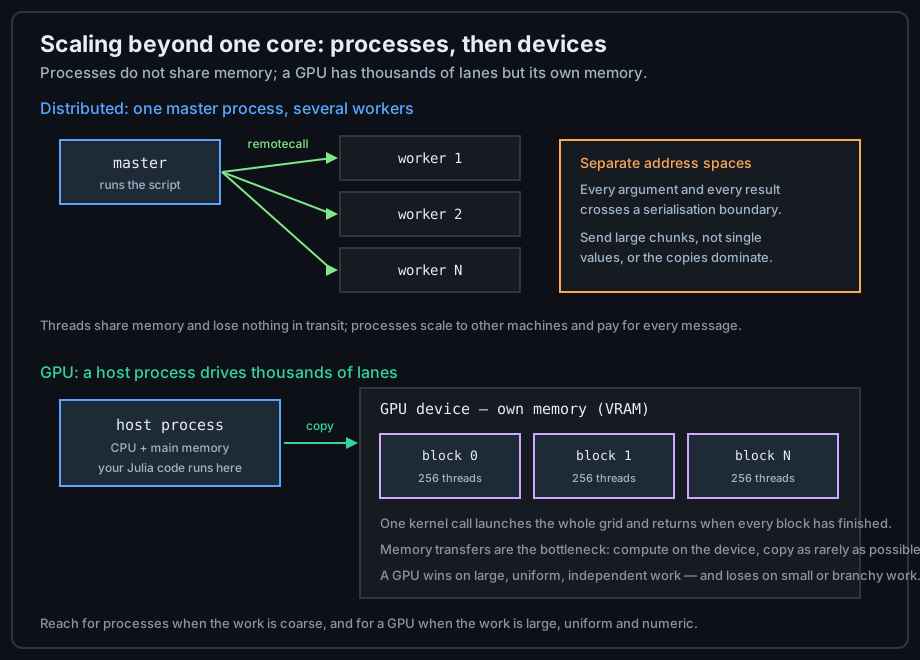
Two facts decide everything that follows: a worker is a separate process with separate memory, and every worker compiles code on first use. Both mean distributed work must be large enough to pay for messages and compilation.

remotecall, fetch, and @spawnat

To run something elsewhere you send a function and its arguments. remotecall returns a Future you fetch later; @spawnat is the macro form; remotecall_fetch does both in one step.

using Distributed

# Run a function on a specific worker and keep the future
f = remotecall(rand, 2, 3)            # worker 2, arguments (3,)
fetch(f)                              # the result: a length-3 vector

# Macro form: pick the worker at the call site
fut = @spawnat 2 sum(1:100)           # a Future on worker 2
fetch(@spawnat 3 6 * 7)               # 42

# Fetch in one call: simplest for small results
remotecall_fetch(+, 2, 1, 2)          # 3

# "Whichever worker is free" — Distributed.@spawn, not Threads.@spawn
t = @spawn sum(rand(1000))
fetch(t)

# Ask every worker for its own id, then collect
futures = [remotecall(myid, w) for w in workers()]
fetch.(futures)                       # [2, 3, 4, 5]

# A failing remote call raises on fetch, like any task
bad = remotecall(error, 2, "remote boom")
# fetch(bad)                          # RemoteException wrapping the error

# Arguments are serialised, so pass a description, not a large payload
remotecall_fetch(n -> sum(1:n), 2, 1_000_000)      # tiny message, big work

Note the argument rule: everything sent to a worker is serialised, so a large array is copied in full. Send a chunk of work over a small description — an index range, a path, a seed — rather than the data itself when the data is large.

@everywhere and Code Loading

A function defined only on the master does not exist on the workers. @everywhere evaluates a definition on every process, which is the first thing to reach for when a remote call reports an undefined function.

using Distributed

# WRONG: defined on the master only
helper(x) = x^2
# remotecall_fetch(helper, 2, 3)      # ERROR: UndefVarError on worker 2

# RIGHT: define it on every process
@everywhere begin
    helper(x) = x^2
    using Statistics                  # imports are per process too
end

remotecall_fetch(helper, 2, 3)        # 9

# @everywhere also loads packages on every worker
@everywhere using LinearAlgebra

# A whole file can be shipped to each worker
for w in workers()
    remotecall_wait(include, w, "worker_setup.jl")
end

# Check what a worker can actually see
remotecall_fetch(() -> names(Main, imported = true), 2)

# The usual script shape: one @everywhere block for definitions,
# then a @distributed loop for the work.

Treat the @everywhere block as the definition section of a distributed program. Everything the workers need — functions, imports, constants — belongs there; anything left out fails only at run time, on a remote process, with a message pointing at the call site.

Distributed Loops and Arrays

Once workers exist, the ordinary way to use them is a parallel loop or a distributed array. The syntax resembles the threaded versions, but the memory boundary changes the performance rules completely.

@distributed Loops and Reductions

@distributed splits a loop's index range across workers. With a + reducer it accumulates partial results; without a reducer it is a for loop that must not return anything.

using Distributed

# A parallel reduction: each worker sums its own range, then they combine
function par_squares(n)
    @distributed (+) for i in 1:n
        i * i                         # the body contributes one value per iteration
    end
end

par_squares(10_000)                   # 333383335000

# Without a reducer the loop runs for its side effects only
@sync @distributed for i in 1:8
    println("i=$i on process $(myid())")
end

# Keep the bodies cheap and local: only the small partials travel back
function par_count(v, pred)
    @distributed (+) for i in eachindex(v)
        pred(v[i]) ? 1 : 0
    end
end

par_count(1:100, iseven)              # 50

# A real workload: each worker computes a slice of a histogram
function par_histogram(v, nbins, lo, hi)
    @distributed (+) for k in 1:nbins
        bin_lo = lo + (k - 1) * (hi - lo) / nbins
        bin_hi = lo + k * (hi - lo) / nbins
        count(x -> bin_lo <= x < bin_hi, v)
    end
end

Every function used by the loop must be defined before it runs — inside the @everywhere block — and the collections it reads should be shared rather than copied. That last point is what the next section is about.

DArrays and SharedArrays

Two array types remove the copying problem in different ways: SharedArray lives in one machine's shared memory and is visible to every local worker, while DArray splits the data across workers, each owning a piece.

using Distributed
@everywhere using SharedArrays

# SharedArray: one array, several processes, shared memory (one machine)
S = SharedArray{Float64}(1000)
@sync @distributed for i in eachindex(S)
    S[i] = sin(i / 100)               # every worker writes into the same array
end
sum(S)                                # a normal reduction on the result

# The master sees the same memory: no gather step is needed
S[1]                                  # sin(0.01)

# DArray: the data itself is partitioned across workers
using DistributedArrays
D = distribute([1.0, 2.0, 3.0, 4.0])  # each worker owns a block
localpart(D)                          # the piece on the current process
Array(D)                              # gather to the master (a copy!)

# Operations run where the data lives, so the master never holds it all
D2 = D .+ 1
Array(D2)                             # [2.0, 3.0, 4.0, 5.0]

# Distributing a large array from the master still copies it once
Dbig = distribute(collect(1:1_000_000))

Choose by where the data lives: SharedArray for one machine with many processes, DArray when the array is too large for one node's memory. On the GPU the same distinction reappears as the host array versus the device array.

pmap and Batch Jobs

pmap applies a function to every element of a collection across workers, sending arguments one at a time. It is the right tool for coarse, independent items — one simulation per parameter set — and the wrong tool for cheap arithmetic.

using Distributed

@everywhere expensive(x) = begin
    s = 0.0
    for k in 1:100_000
        s += sin(k * x)
    end
    s
end

# One task per element, spread over the workers
pmap(expensive, 1:8)                  # eight values, computed on the cluster

# pmap keeps the input order in the output, like map
results = pmap(x -> (x, x^2), 1:5)
results                               # [(1,1), (2,4), ...] in order

# batch_size controls how many elements each message carries
pmap(expensive, 1:100; batch_size = 10)      # fewer, larger messages

# on_error lets one bad element fail without losing the whole run
pmap(x -> x == 3 ? error("bad") : x, 1:4; on_error = identity)

# When per-element work is tiny, use a @distributed loop instead:
# pmap pays message overhead on every element.

Use pmap when the work per item is measured in seconds, not microseconds. For anything smaller, @distributed over index ranges carries far less message overhead.

The GPU Model

A graphics card is not a faster CPU. It is thousands of simple lanes that must all execute the same instruction on different data, behind a memory bus that is fast but narrow. Everything surprising about GPU programming follows from those two facts.

Why a GPU Is Different

Where a CPU has a few complex cores with large caches, a GPU has thousands of lanes sharing a scheduler and a wide memory interface. It rewards uniformity and punishes divergence, and its memory is separate from the host's.

# The mental model in three lines
#   CPU: few cores, deep caches, branch prediction, low latency per instruction
#   GPU: many lanes, wide memory bandwidth, high throughput, no per-lane caching
#   Host and device do NOT share memory: data must be copied over the bus

# A task is worth a GPU when it is:
#   - large        (millions of elements, or a big matrix)
#   - uniform      (the same operation applied to every element)
#   - independent  (no element depends on another's intermediate value)
#   - numeric      (floating point, integers, or small fixed-size structs)

# Maps well: array arithmetic, matrix multiply, stencils, convolutions,
# Monte Carlo sampling, dense linear algebra.
# Maps badly: parsing, pointer chasing, branchy logic, and anything with
# a small amount of computation and a large amount of setup.

The first thing to check before porting code is whether it is already limited by memory bandwidth rather than arithmetic. If it is, a GPU helps less than you expect — both machines are waiting on the same kind of resource.

GPU Arrays and Unified Memory

Packages such as CUDA.jl give you an array type that lives on the device. Operations on a CuArray compile to GPU code, while Array brings the data back to the host — and that conversion is where most of the time goes.

using CUDA

# Check the device and its memory before doing anything else
CUDA.functional()                     # is a GPU available and usable?
CUDA.name(CUDA.device())              # e.g. "NVIDIA ..."
CUDA.available_memory()               # bytes free on the device

# Move data to the device: this is the expensive step
h = rand(Float32, 1024, 1024)         # host array (CPU memory)
d = CuArray(h)                        # device array (VRAM) — copies

# Operations now run on the device, element-wise and in parallel
d2 = d .* 2 .+ 1                      # a CuArray again
sum(d2)                               # a GPU reduction

# Bring a result back only when you need it on the host
result = Array(d2)[1:3]               # a copy back to CPU memory

# Prefer Float32 on the GPU: faster than Float64 and usually accurate enough
# 1024x1024 Float64 → 8 MB per array; Float32 → 4 MB

# Reuse device buffers to avoid repeated allocation and transfer
buf = CUDA.zeros(Float32, 1024, 1024)
copyto!(buf, h)                       # transfer into an existing buffer
buf .= buf .* 2.0f0                   # in-place: no new allocation

Write the algorithm once for the host array, then wrap it in a function whose argument type decides where it runs. A generic function with Float32 data and dotted operations works on a CuArray unchanged, which is how one source serves both CPU and GPU.

Kernels and the Thread Hierarchy

When broadcasting is not enough — when a computation needs an index, a shared buffer, or an inner loop — you write a kernel. A kernel is a function executed by many threads at once, each identified by its position in the grid.

using CUDA

# A kernel: one thread per output element, identified by its index
function double_kernel!(out, inp)
    i = (blockIdx().x - 1) * blockDim().x + threadIdx().x
    if i <= length(out)
        @inbounds out[i] = 2 * inp[i]
    end
    return nothing
end

n = 1024
d_out = CUDA.zeros(Float32, n)
d_inp = CUDA.ones(Float32, n)

# Launch: threads = block size, blocks = how many blocks cover n
threads = 256
blocks = cld(n, threads)
@cuda threads = threads blocks = blocks double_kernel!(d_out, d_inp)
Array(d_out)[1:3]                     # [2.0, 2.0, 2.0]

# A kernel that needs neighbouring values must synchronise
function stencil_kernel!(out, inp)
    i = (blockIdx().x - 1) * blockDim().x + threadIdx().x
    shared = @cuStaticSharedMem(Float32, 256)     # fast memory shared per block
    shared[threadIdx().x] = inp[i]
    sync_threads()                                # wait for all writes
    if 1 < threadIdx().x <= 256
        @inbounds out[i] = 0.5f0 * (shared[threadIdx().x - 1] + shared[threadIdx().x])
    end
    return nothing
end

@cuda threads = 256 blocks = cld(n, 256) stencil_kernel!(d_out, d_inp)

Two rules keep kernels correct: every thread must return something (usually nothing) and must guard its index against the array bounds, because the last block is usually partial; and any value shared between threads needs an explicit sync_threads() before it is read.

GPU Programming in Practice

Most useful GPU code never leaves Julia's ordinary syntax. Start from broadcasting, drop to a kernel only where broadcasting cannot express the computation, and measure the transfers — they are usually the real bottleneck.

Broadcasting on the GPU

Dotted expressions are the first and often the last tool you need. Each broadcast is one kernel launch, and fusing the dots into a single expression keeps intermediate values on the device.

using CUDA

# One broadcast chain, one kernel, no host round trip
function normalise!(d)
    d .-= sum(d) / length(d)                       # mean centring on the device
    d ./= (maximum(abs, d) + eps(Float32))         # scale in place
    d
end

d = CuArray(rand(Float32, 1024, 1024))
normalise!(d)

# Fuse the dots: separate statements write intermediates to VRAM twice
a = CUDA.ones(Float32, 1_000_000)
b = CUDA.ones(Float32, 1_000_000)
c = 2 .* a .+ 3 .* b                 # one fused kernel, one result array
# slow alternative: x = 2 .* a; y = 3 .* b; c = x .+ y  (three arrays)

# Views keep their parent on the device: no copy, no transfer
row = @view d[1, :]
sum(row)                             # a GPU reduction over a view

# Generic functions work for both host and device inputs
function scale_all!(v, k)
    v .= k .* v
    v
end

scale_all!(rand(Float32, 4), 2.0f0)              # CPU array
scale_all!(CUDA.ones(Float32, 4), 2.0f0)         # GPU array — same source

The rule is the same as on the CPU, with higher stakes: fewer, larger operations. Twenty small broadcasts cost twenty kernel launches, and on a GPU the launch overhead is comparable to the work for small arrays.

Writing a Kernel

A custom kernel earns its place when the computation has a structure the broadcast machinery cannot see: a neighbour dependency, a block-level reduction, or an index-based loop. Start from the broadcasting version and replace only the part that does not fit.

using CUDA

# Kernel with a guard: y = a*x + b, one thread per element
function saxpby_kernel!(y, a, x, b, n)
    i = (blockIdx().x - 1) * blockDim().x + threadIdx().x
    if i <= n
        @inbounds y[i] = a * x[i] + b
    end
    return nothing
end

function saxpby!(y, a, x, b)
    n = length(y)
    threads = 256
    blocks = cld(n, threads)
    @cuda threads = threads blocks = blocks saxpby_kernel!(y, a, x, b, n)
    y
end

n = 1_000_000
x = CUDA.ones(Float32, n)
y = CUDA.zeros(Float32, n)
saxpby!(y, 2.0f0, x, 1.0f0)
Array(y)[1]                          # 3.0

# Test the kernel with a tiny array first — errors are easier to see
small_x = CUDA.ones(Float32, 5)
small_y = CUDA.zeros(Float32, 5)
saxpby!(small_y, 2.0f0, small_x, 1.0f0)
Array(small_y)                       # [3.0, 3.0, 3.0, 3.0, 3.0]

# KernelAbstractions lets one kernel run on any backend
#   using KernelAbstractions
#   @kernel function scale_kernel!(v, k)
#       i = @index(Global, Linear)
#       @inbounds v[i] *= k
#   end
#   kernel!(CPU())(v, 2.0f0; ndrange = length(v))

Always test a kernel against a small CPU implementation before trusting it on a million elements. A wrong index computation reads out of bounds silently, and on a GPU that shows up as a wrong number rather than a crash on the offending line.

Transfers and the Waterfall

The bus is the bottleneck, so the winning strategy is to move data across it as rarely as possible. Keep arrays resident on the device and combine steps into one round trip instead of several.

using CUDA

# BAD: three host/device round trips for one computation
function slow_roundtrip(h)
    a = CuArray(h)
    b = Array(a .* 2)                # back to the host...
    c = CuArray(b .+ 1)              # ...and out again
    sum(c)
end

# GOOD: everything happens on the device, one transfer at the end
function fast_resident(h)
    d = CuArray(h)                   # one transfer in
    d .= d .* 2 .+ 1                 # no transfer at all
    sum(d)                           # a single scalar comes back
end

using BenchmarkTools
@btime slow_roundtrip($(rand(Float32, 1_000_000)))
@btime fast_resident($(rand(Float32, 1_000_000)))

# Timing a GPU operation needs a synchronisation, or you time the launch only
CUDA.@time (d = CUDA.ones(Float32, 10_000_000); sum(d))
CUDA.synchronize()                   # wait for the device to finish

# Pinned host memory makes transfers faster when they are unavoidable
# p = CUDA.Mem.alloc(CUDA.Mem.HostBuffer, nbytes)

# Small frequent transfers are the worst case: batch them.
#   Move 100 arrays at once, not one array 100 times.

Measure with a synchronisation, or you will time the asynchronous launch rather than the computation. And remember the rule that explains most disappointing GPU results: an algorithm with little computation per byte transferred is dominated by the bus, not the device.

Pitfalls of Scale-Out

Scaling out multiplies the cost of every mistake: a slow message is paid by every worker, and a wrong kernel is paid by a million threads. These are the failures worth designing against.

Serialisation and Grain Size

Every message between processes is serialised, sent, and deserialised. If the work per message is smaller than that cost, adding workers makes the program slower — the same overhead trap as threading, at a much higher price per unit.

using Distributed

# BAD: one message per element, each carrying real data
function tiny_tasks(v, ws = workers())
    [remotecall_fetch(x -> x^2, ws[mod1(i, length(ws))], v[i]) for i in eachindex(v)]
end

# GOOD: one message per worker, carrying a range
function coarse_tasks(v)
    n = length(v)
    step = cld(n, nworkers())
    futures = [remotecall_fetch(ks -> sum(x -> x^2, @view v[ks]), w, k:min(k + step - 1, n))
               for (k, w) in zip(1:step:n, workers())]
    sum(futures)
end

# The size of the DATA matters more than the count of messages
#   sending  1 KB   → the message overhead dominates
#   sending  1 MB   → the serialisation dominates
#   sending 10 MB   → you should be reading it on the worker instead

# Prefer a path or a specification over a payload
full_input = rand(1000, 1000)
remotecall_fetch(path -> sum(read(path)), 2, "data.bin")     # small message

# Measure the cost of the boundary itself
using BenchmarkTools
@btime remotecall_fetch(sum, 2, $(rand(10_000)))             # includes serialisation

Design distributed work in chunks of seconds, not milliseconds, and move the data once. A job whose messages outweigh its computation is a single-machine job wearing a distributed costume.

Portability and Vendor Lock

CUDA runs on NVIDIA hardware; AMD and Intel need different packages. The escape is to write against an abstraction that has backends, so the same source runs on any accelerator available.

# Choose the array type by the hardware you actually have
#   CUDA.jl      → NVIDIA GPUs        (CuArray)
#   AMDGPU.jl    → AMD GPUs           (ROCArray)
#   oneAPI.jl    → Intel GPUs         (oneArray)
#   Metal.jl     → Apple silicon      (MtlArray)

# Write the kernel against KernelAbstractions and pick the backend at run time
using KernelAbstractions

@kernel function saxpy_kernel!(y, a, x)
    i = @index(Global, Linear)
    @inbounds y[i] = a * x[i]
end

function saxpy!(backend, y, a, x)
    kernel! = saxpy_kernel!(backend, 256)
    kernel!(y, a, x; ndrange = length(y))
end

# One implementation, several backends — the choice becomes configuration
# backend = CUDABackend()  # or ROCBackend(), oneAPIBackend(), CPU()

# For portable array code, prefer the vendor-neutral array package
#   using GPUArrays
#   # functions written for AbstractGPUArray run on any of them

# Test on the CPU backend in CI: no GPU needed to catch index errors
@assert saxpy!(CPU(), [1.0, 2.0], 2.0, [1.0, 1.0]) == [2.0, 4.0]

Write the kernel once with KernelAbstractions, keep a CPU backend for tests, and let deployment decide which accelerator runs it. That is also the only way to test GPU-shaped code on a machine without a GPU.

Testing at Scale

Parallel and device code must be tested the same way as any other code — against a known-correct reference. The trick is to keep the reference sequential, and to make the parallel path equal to it exactly.

using Distributed, Test

# A sequential reference implementation lives beside the parallel one
seq_sum(v) = sum(x -> x^2, v)

@everywhere par_chunk(ks) = sum(x -> x^2, ks)

function par_sum(v)
    n = length(v)
    step = cld(n, nworkers())
    parts = [remotecall_fetch(par_chunk, w, k:min(k + step - 1, n))
             for (k, w) in zip(1:step:n, workers())]
    sum(parts)
end

@testset "distributed sums match the sequential reference" begin
    for n in (0, 1, 7, 100, 10_000)
        v = collect(1:n)
        @test par_sum(v) == seq_sum(v)
    end
end

# Boundary cases are where distributed bugs hide
@test par_sum(Int[]) == 0            # empty input: no chunks at all
@test par_sum([1]) == 1              # fewer elements than workers

# For a GPU kernel, the same idea with the CPU implementation as reference
#   @test Array(gpu_result) ≈ cpu_result
# The comparison is approximate: floating-point order differs on the device.

# Deterministic reduction order keeps the result reproducible run to run
# (a floating-point sum that depends on thread order will drift).

Two habits make scaled code trustworthy: an exact test at the small sizes where the chunking logic is exercised, and an approximate comparison for floating-point results, where the order of additions legitimately differs.

Choosing to Scale

Scaling is a decision with costs on both sides: development time, debugging difficulty, reproducibility, and often money. The honest question is not "can this run in parallel" but "does the speedup justify what it costs to maintain".

Size Matters

Both forms of scale-out are only worth it above a size where the overhead disappears. Measuring that threshold on your own hardware takes minutes and prevents months of over-engineering.

# The threshold test: measure the same function at growing sizes,
# sequentially and in parallel, and find where the curves cross.
using BenchmarkTools, Distributed

function crossover(f, sizes)
    for n in sizes
        x = rand(n)
        t1 = @belapsed $f($x)
        nprocs() > 1 || continue
        t2 = @belapsed pmap($f, x)
        println(rpad(n, 10), round(t1 * 1e6, digits = 1), " μs seq   ",
                round(t2 * 1e6, digits = 1), " μs par")
    end
end

# Typical outcome for a cheap function: parallel is SLOWER until ~10^5 elements
# crossover(sum, (100, 1_000, 10_000, 100_000, 1_000_000))

# For a GPU the threshold is higher still: transfers alone cost milliseconds,
# so a device only wins above roughly 10^6 elements (or a dense matrix operation).

# Rules of thumb worth remembering
#   threads   → from ~10 μs of work per chunk
#   processes → from ~10 ms of work per message
#   GPU       → from ~1 ms of device-resident work, on large uniform arrays

# And the fallback that always works: fix the types and the allocations first
# (the previous lesson). A 20× single-thread win costs nothing to maintain.

Exhaust the single-machine options before scaling out: type stability, allocations, and loop order usually deliver the largest improvement for the least complexity. Parallelism is what you do after the sequential code is already good.

Cluster and Cloud Setup

The same Distributed API works on a cluster — only the way workers appear changes. A cluster manager hands you processes, and your script is unchanged apart from the addprocs call.

# On a Slurm cluster
#   using Distributed, SlurmClusterManager
#   addprocs(SlurmManager(); partition = "gpu", ntasks = 16, ntasks_per_node = 4)

# With ssh-accessible machines, no manager is needed
#   addprocs(["node1", "node2"], sshflags = "-i ~/.ssh/id_rsa")

# Recipe for a portable job script
using Distributed

function main()
    n = nworkers()
    n > 1 || error("start with workers: julia -p 8 script.jl")
    @everywhere begin
        using Statistics                 # everything workers need, on every worker
        heavy(x) = mean(sin.(x .* (1:1000)))
    end
    results = pmap(heavy, [rand(10_000) for _ in 1:n])
    (workers = n, mean = mean(results))
end

main()

# In containers the same rules as threading apply: declare the CPU and GPU
# resources you expect, and make the worker count explicit.

# Checkpoint long jobs: a cluster job that dies at hour nine should not
# restart from zero. Write partial results with Serialization.
using Serialization
serialize("checkpoint.jls", results)             # write
results = deserialize("checkpoint.jls")          # read

Keep the job script free of machine-specific assumptions: worker count from the command line, resources declared at submission, and results checkpointed so a failure costs minutes instead of hours.

The Cost of Scale

Every additional layer of parallelism adds a failure mode, a debugging difficulty, and often a bill. Senior work is knowing when to stop — and being able to explain the trade-off in numbers.

# Write the justification down, in the code, next to the implementation.
# It is the cheapest documentation you will ever produce.

#   Problem:   fit 500 models, 4 s each, single-threaded  → 33 minutes
#   Option A:  threads -t 8 → 4.2 minutes, no extra infrastructure
#   Option B:  GPU → 1.5 minutes, but requires a device and a rewrite
#   Decision:  Option A. B's extra 3 minutes do not pay for the portability
#              loss and the CI cost.
#   Boundary:  revisit if the model count exceeds 5 000.

# Questions to answer before scaling out:
#   - What is the sequential time, measured, on the real input?
#   - What fraction of it can be parallelised? (Amdahl's ceiling)
#   - What does each layer cost in complexity: threads < processes < GPU?
#   - Can the sequential version be made fast instead? (types, allocations)
#   - How will this be tested, and on what hardware, in CI?

# And the invariants that must hold at every scale
@assert sum(1:1000) == 500500                 # the reference result
# @test parallel_version(input) == reference(input)   # in your test suite

A performance decision that cannot be explained with three numbers and a boundary condition will be reversed by the next person who reads it. Write the numbers down — measured, dated, with the hardware they came from.

All of the work in this lesson assumes Julia itself; the code around it lives elsewhere. Next: Interop covers calling C, Fortran, and Python from Julia — and calling Julia from them.