
Optimization & JuMP
The lesson is organised by problem class, because the class decides everything: which solver can be used, whether the answer is guaranteed optimal, and how long the search will take. Linear and convex problems are solved to proven optimality in seconds; a mixed-integer or non-convex problem may consume an hour and still return "feasible, not proven optimal". Knowing which one you are writing is the difference between a tool and a lottery.
The lesson is organised by problem class, because the class decides everything: which solver can be used, whether the answer is guaranteed optimal, and how long the search will take. Linear and convex problems are solved to proven optimality in seconds; a mixed-integer or non-convex problem may consume an hour and still return "feasible, not proven optimal". Knowing which one you are writing is the difference between a tool and a lottery.
Optimization in Julia
Begin with the classification, because it constrains every later choice.
Problem Classes
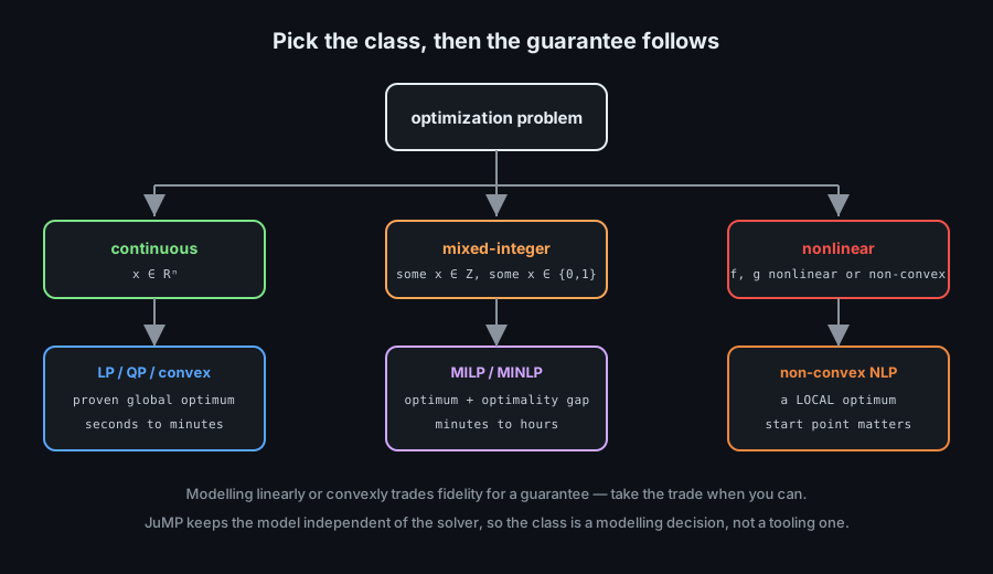
Each class is defined by the shape of the objective and the constraints. The shape determines what a solver can promise you.
| Class | Objective and constraints | What a solver can promise |
|---|---|---|
| LP — linear programming | Linear both | A proven global optimum, fast, in polynomial time |
| MILP — mixed-integer linear | Linear, some variables integer | Global optimum or a bound on how far the incumbent is from it |
| QP / convex | Convex objective, convex constraints | Global optimum; any local solution is the global one |
| NLP — nonlinear | Arbitrary smooth functions | Usually a local optimum only |
| Non-convex / combinatorial | Discrete structure, many local optima | Nothing general — a good answer and no guarantee |
The practical reading: if you can state the problem linearly or convexly, do that. You exchange modelling freedom for a guarantee, and the guarantee is usually worth more than the fidelity.
The Ecosystem
Julia separates the model from the solver. One model file, many solvers — the same code runs on an open-source solver on your laptop and a commercial one on the cluster.
# The layers
#   JuMP.jl        → the modelling language (variables, constraints, objective)
#   MathOptInterface → the interface both JuMP and solvers speak
#   a solver       → the arithmetic: HiGHS, GLPK, Ipopt, Cbc, Gurobi, CPLEX

using JuMP
using HiGHS                # open source LP/MILP solver
using Ipopt                # open source nonlinear solver

# A solver choice is one line — the model above it does not change
model = Model(HiGHS.Optimizer)
model = Model(Ipopt.Optimizer)
# model = Model(Gurobi.Optimizer)          # same model, a commercial solver

# Look at what is available in this environment
#   ] add JuMP HiGHS Ipopt
#   using JuMP; JuMP.installed_solvers()
This separation is the reason JuMP is worth learning instead of a solver's own API: a model that took a day to write is not tied to a licence, a vendor, or a version.
Objective Functions and Feasibility
Every optimization problem has the same three parts. State them explicitly before writing code — the discipline prevents most modelling errors.
# The three parts, in words first:
#
#   DECISION VARIABLES  what we choose       x₁, x₂ ≥ 0
#   OBJECTIVE           what we want         minimise  3x₁ + 2x₂
#   CONSTRAINTS         what is allowed      x₁ + x₂ ≥ 10
#                                           2x₁ +  x₂ ≥ 12
#
# In JuMP:

using JuMP, HiGHS

model = Model(HiGHS.Optimizer)

@variable(model, x1 >= 0)
@variable(model, x2 >= 0)

@objective(model, Min, 3x1 + 2x2)

@constraint(model, c1, x1 + x2 >= 10)
@constraint(model, c2, 2x1 + x2 >= 12)

optimize!(model)

termination_status(model)      # OPTIMAL
objective_value(model)         # 24.0
value(x1), value(x2)           # (2.0, 8.0)

# Always check the status before reading values: a failed solve also has
# an incumbent, and it is usually nonsense.
Naming constraints (c1, c2) costs nothing and pays immediately: solvers report infeasibility and dual values by name, and a name is far easier to act on than "row 7".
Linear Programming with JuMP
An LP is the friendliest problem in optimization: any local optimum is global, the answer is exact, and a solver will prove it. Most production planning models are LPs or nearly so.
Building a Production Model
A realistic example: choose production quantities for several products to maximise profit, subject to machine hours and demand limits.
using JuMP, HiGHS

# Data
products   = [:widget, :gadget, :sprocket]
profit     = Dict(:widget => 12.0, :gadget => 9.0, :sprocket => 15.0)
hours      = Dict(:widget => 0.5,  :gadget => 1.0, :sprocket => 1.5)   # per unit
demand_max = Dict(:widget => 100,  :gadget => 120, :sprocket => 60)
machine_hours = 200.0

model = Model(HiGHS.Optimizer)
set_silent(model)

# Continuous variables with bounds, created from data — no copy-paste
@variable(model, 0 <= x[p in products] <= demand_max[p])

# Objective: total profit, written as a sum over the index set
@objective(model, Max, sum(profit[p] * x[p] for p in products))

# Constraint: the shared resource
@constraint(model, machine_use, sum(hours[p] * x[p] for p in products) <= machine_hours)

optimize!(model)

termination_status(model)          # OPTIMAL
objective_value(model)             # the maximum profit
value.(x)                          # the quantities, one per product
value(machine_use)                 # hours actually used
dual(machine_use)                  # the shadow price of one extra hour
The dual of the resource constraint is the number a manager actually wants: the increase in profit per additional machine hour. It is free to compute and it answers the question everyone asks after "what is the optimum?".
Constraints, Bounds and Index Sets
Real models have constraints per product, per period, or per pair. JuMP expresses them as comprehensions over index sets, not loops of copy-pasted lines.
using JuMP, HiGHS

model = Model(HiGHS.Optimizer)

weeks = 1:4
items = [:a, :b]

@variable(model, x[i in items, t in weeks] >= 0)
@variable(model, 0 <= inv[i in items, t in weeks] <= 50)

# Inventory balance: stock carries over, demand is met from stock
demand = Dict((:a, 1) => 10, (:a, 2) => 12, (:b, 1) => 8, (:b, 2) => 9)
@constraint(model, balance[i in items, t in weeks],
    inv[i, t] == x[i, t] + (t == first(weeks) ? 0 : inv[i, t-1]) - get(demand, (i, t), 0)
)

# Capacity that links items: total production per week is limited
@constraint(model, cap[t in weeks], sum(x[i, t] for i in items) <= 30)

# Absolute value via two linear inequalities — the standard trick
@variable(model, deviation[t in weeks] >= 0)
@constraint(model, dev_pos[t in weeks], deviation[t] >= x[:a, t] - 15)
@constraint(model, dev_neg[t in weeks], deviation[t] >= 15 - x[:a, t])

# Every constraint and variable is named and enumerable
num_variables(model)
num_constraints(model; count_variable_in_set_constraints = false)
The inventory-balance constraint shows how a t == first(weeks) conditional keeps an initial condition inside the same formula. That avoids an off-by-one bug that is otherwise invisible until the model reports an impossible optimum.
Solving and Interpreting Results
Reading a solution properly means reading the status, the objective, the variables, and the duals — in that order.
using JuMP, HiGHS

optimize!(model)

# 1. Status first — everything else depends on it
termination_status(model)         # OPTIMAL | INFEASIBLE | DUAL_INFEASIBLE | TIME_LIMIT | ...
primal_status(model)              # FEASIBLE_POINT | NO_SOLUTION
dual_status(model)

if termination_status(model) == MOI.OPTIMAL
    @info "solved" profit = objective_value(model) hours = value(machine_use)
elseif termination_status(model) == MOI.INFEASIBLE
    # Ask the solver which constraints conflict
    compute_conflict!(model)
    for (F, S) in list_of_constraint_types(model)
        for con in all_constraints(model, F, S)
            if MOI.get(model, MOI.ConstraintConflictStatus(), con) != MOI.NOT_IN_CONFLICT
                @warn "conflicting constraint" name = name(con)
            end
        end
    end
end

# 2. Sensitivity: what would one more unit of the resource be worth?
dual(machine_use)                 # shadow price
reduced_cost(x[:widget])          # how far this product is from being worth making

# 3. Solution quality when there is no guarantee
objective_value(model)            # the incumbent
MOI.get(model, MOI.RelativeGap()) # for MIP: how far from proven optimal
compute_conflict! is the single most useful debugging tool in LP work. "Infeasible" alone tells you nothing; a list of the constraints that cannot hold together tells you exactly which business rule contradicts which.
Integer and Mixed-Integer Programming
The moment a variable must be an integer — a number of machines, a yes/no decision — the problem becomes combinatorial and the guarantee changes shape.
Binary and Integer Variables
Two variable kinds cover almost every discrete model: an integer count and a binary on/off switch.
using JuMP, HiGHS

model = Model(HiGHS.Optimizer)

# Integer counts (units produced, trucks used, staff scheduled)
@variable(model, n_machines >= 0, Int)

# Binary decisions (open a facility, assign a task, select a candidate)
@variable(model, open_a, Bin)
@variable(model, open_b, Bin)

# The standard big-M link: produce only if the facility is open
M = 1000.0
@variable(model, 0 <= output_a <= M * open_a)
@variable(model, 0 <= output_b <= M * open_b)

# Fixed cost plus variable cost
fixed  = 500.0
margin = 3.0
@objective(model, Max, margin * (output_a + output_b) - fixed * (open_a + open_b))

@constraint(model, demand, output_a + output_b >= 120)

optimize!(model)

# Check how close the answer is to PROVEN optimal
gap = MOI.get(model, MOI.RelativeGap())        # 0.0 means proven optimal
@info "MIP result" profit = objective_value(model) gap = gap open = (value(open_a), value(open_b))
Choose M as tightly as the data allows. A big-M far larger than the real capacity makes the linear relaxation very weak, and a weak relaxation is why a MIP that should take a second takes an hour.
Scheduling and Assignment Models
The assignment model is the canonical integer program: match workers to shifts, tasks to machines, items to bins — one matrix of binaries and one constraint per row and per column.
using JuMP, HiGHS

workers = [:ana, :bogdan, :carla]
shifts  = [:mon, :tue, :wed]
cost = Dict((:ana, :mon) => 10, (:ana, :tue) => 12, (:ana, :wed) => 11,
            (:bogdan, :mon) => 9, (:bogdan, :tue) => 14, (:bogdan, :wed) => 10,
            (:carla, :mon) => 8, (:carla, :tue) => 9,  (:carla, :wed) => 12)

model = Model(HiGHS.Optimizer)

# x[w, s] = 1 when worker w covers shift s
@variable(model, x[w in workers, s in shifts], Bin)

# Each shift covered exactly once
@constraint(model, cover[s in shifts], sum(x[w, s] for w in workers) == 1)

# Each worker takes at most two shifts
@constraint(model, load[w in workers], sum(x[w, s] for s in shifts) <= 2)

# No worker on both Tuesday and Wednesday (a fairness rule)
@constraint(model, no_consecutive[w in workers], x[w, :tue] + x[w, :wed] <= 1)

@objective(model, Min, sum(cost[(w, s)] * x[w, s] for w in workers, s in shifts))

optimize!(model)

if termination_status(model) == MOI.OPTIMAL
    for s in shifts
        w = only(w for w in workers if value(x[w, s]) > 0.5)
        println(s, " → ", w)
    end
end

# Extracting the solution back into a data structure is part of the model:
# a solution nobody can read is a solution nobody will act on.
Note the shape of the extraction loop: from a matrix of binaries to a plain list of assignments. That conversion is where domain rules get re-checked before anybody trusts the schedule.
MIP Pitfalls
Integer programs fail in ways that look like solver bugs but are almost always modelling problems.
| Symptom | Cause | Fix |
|---|---|---|
| Solve runs for hours | Weak LP relaxation from a huge big-M | Tighten M to the real bound |
| No feasible solution found | An equality constraint is over-restrictive | Relax to <=/>=, or run compute_conflict! |
| Solution is fractional | Variables declared continuous by accident | Add Int or Bin and re-check the values |
| Memory exhausted | Too many binaries (thousands × thousands) | Reformulate: aggregate, add valid inequalities, drop symmetry |
| Equivalent optima, different answers daily | Symmetry in the model | Add a symmetry-breaking constraint |
| Answer differs from a colleague's | Different solver version or gap tolerance | Record solver, version, and RelativeGap with the result |
The last row is the practical reason to log solver settings: an integer program has no unique "the answer" unless the optimality gap is zero, and two runs at different tolerances legitimately differ.
Nonlinear and Convex Optimization
When the objective or a constraint is nonlinear, the guarantees change — and the model class you choose decides whether you get the global optimum or a local one.
Optim.jl and Roots.jl
For unconstrained or simply-constrained nonlinear problems, Optim.jl is lighter than JuMP and gives you direct control over the algorithm.
using Optim

# Unconstrained: the Rosenbrock function with the classic valley
rosenbrock(x) = (1.0 - x[1])^2 + 100.0 * (x[2] - x[1]^2)^2

result = optimize(rosenbrock, [-1.2, 1.0], NelderMead())
result = optimize(rosenbrock, [-1.2, 1.0], BFGS())          # needs a gradient
result = optimize(rosenbrock, [-1.2, 1.0], LBFGS())         # limited-memory BFGS

Optim.minimizer(result)     # the point found
Optim.minimum(result)       # the function value there

# Supplying the gradient yourself is faster and more accurate
function rosenbrock_g!(G, x)
    G[1] = -2(1 - x[1]) - 400x[1]*(x[2] - x[1]^2)
    G[2] = 200(x[2] - x[1]^2)
    return G
end
optimize(rosenbrock, rosenbrock_g!, [-1.2, 1.0], BFGS())

# Or let automatic differentiation do it
using ForwardDiff
optimize(rosenbrock, [-1.2, 1.0], BFGS(); autodiff = :forward)

# Box constraints
optimize(rosenbrock, [0.0, 0.0], [1.0, 1.0], [0.5, 0.5], Fminbox(LBFGS()))

# Root finding is the one-dimensional cousin
using Roots
find_zero(x -> x^3 - 2x - 5, 2.0)          # a root near 2
find_zero(sin, (3.0, 4.0))                 # bracketed
The distinction to carry forward: Optim.jl solves the mathematical problem directly, while JuMP is for problems you want to express declaratively and solve with an industrial solver. Both are normal Julia code; there is no wrong choice, only a fit.
Nonlinear Models in JuMP
JuMP handles nonlinear expressions directly: write the function as you would in Julia, and give the solver a starting point.
using JuMP, Ipopt

model = Model(Ipopt.Optimizer)
set_silent(model)

@variable(model, 0.1 <= x <= 10, start = 1.0)
@variable(model, 0.1 <= y <= 10, start = 1.0)

# A nonlinear objective: a cost curve with economies of scale
@objective(model, Min, 100 / x + 50 / y + 2 * x + 3 * y)

# A nonlinear constraint: the production function
@constraint(model, production, x^0.6 * y^0.4 >= 8)

# A squared-slack form keeps ill-conditioned constraints well behaved
@variable(model, slack >= 0)
@constraint(model, smooth, slack^2 == x^2 + y^2 - 20)

optimize!(model)

termination_status(model)     # LOCALLY_SOLVED for a non-convex model
value(x), value(y)

# The starting point is part of the model
set_start_value(x, 5.0)
set_start_value(y, 2.0)

# For a non-convex objective, run from several starts and compare
using Random
best = nothing
for seed in 1:10
    Random.seed!(seed)
    set_start_value(x, rand() * 10)
    set_start_value(y, rand() * 10)
    optimize!(model)
    if termination_status(model) == MOI.LOCALLY_SOLVED
        v = objective_value(model)
        best = isnothing(best) || v < best.value ? (value = v, x = value(x), y = value(y)) : best
    end
end
The multi-start loop is the honest answer to non-convexity. There is no algorithm that finds the global optimum of an arbitrary nonlinear function, so the practical strategy is many starts plus proof that the best of them is stable under perturbation.
Gradients, AD and Solver Tuning
Solver performance in nonlinear work is dominated by derivative information, and Julia can supply it automatically.
using JuMP, Ipopt, ForwardDiff, Enzyme

# JuMP can differentiate the model itself
set_attribute(model, "hessian_approximation", "limited-memory")

# Or register derivatives explicitly for a custom function
f(x) = exp(-x[1]^2 - x[2]^2)
register(model, :f, 2, f; autodiff = true)

# Automatic differentiation packages, by use case
#   ForwardDiff.jl   → forward mode: best for few inputs, many outputs
#   ReverseDiff.jl   → reverse mode: best for many inputs, one output (gradients)
#   Enzyme.jl        → reverse mode on compiled code, very fast, handles mutation

using ForwardDiff
g = ForwardDiff.gradient(f, [1.0, 2.0])
H = ForwardDiff.hessian(f, [1.0, 2.0])

# Tolerance and iteration settings — record them with the result
set_optimizer_attribute(model, "tol", 1e-8)
set_optimizer_attribute(model, "max_iter", 3000)
set_optimizer_attribute(model, "print_level", 0)

# Reading the report is part of solving
raw_status(model)                       # "Solve_Succeeded"
dual_status(model)                      # are the multipliers available?
result_count(model)                     # > 1 means several solutions were returned
objective_value(model; result = 2)      # inspect the alternative
result_count(model) is easy to overlook and occasionally saves a week: when a solver returns several solutions, the first is not necessarily the one your colleagues expect, and the alternatives are often a better trade-off in practice.
Convex Modelling
A convex problem has one property that changes everything: every local optimum is the global optimum. If a problem can be reformulated as convex without inventing lies about the world, that reformulation is the most valuable line of code in the project.
Convex.jl and Disciplined Programming
Convex.jl enforces convexity as you write, by refusing expressions that break the rules. That refusal is the feature.
using Convex, SCS

# Variables
x = Variable(3)

# A convex objective: least squares
A = randn(10, 3); b = randn(10)
problem = minimize(sumsquares(A * x - b))
solve!(problem, SCS.Optimizer)
evaluate(x)

# Norms and penalties are first-class
problem = minimize(norm(A * x - b, 2) + 0.1 * norm(x, 1))     # L2 + L1
solve!(problem, SCS.Optimizer)

# Constraints build the feasible set
problem = minimize(sumsquares(x - [1.0, 2.0, 3.0]),
                   [ sum(x) == 1, x >= 0 ])

# Convex.jl refuses non-convex expressions at construction time:
#   maximize(sin(x[1]))         # ERROR: sin is not convex or concave
#   minimize(x[1] * x[2])       # ERROR: the product of two variables is not convex

# Status and solution
problem.status                # OPTIMAL | INFEASIBLE | UNBOUNDED
problem.optval                # the optimal objective value
evaluate(x)                   # the optimal point
Reading a "not convex" error as a modelling message rather than an API quirk is the skill here. It means the problem as stated has multiple local optima, and the answer you get will depend on where the solver started.
Recognising and Using Convexity
Three practical tests decide whether a formulation is convex, and each one has a standard repair when it fails.
# 1. Objective: sum of convex functions is convex.
#    ||Ax - b||², ||x||₂, ||x||₁, max(x, 0), exp(x), -log(x) are convex.
#    -log(x) is convex for x > 0 — which is why log-likelihood
#    maximisation becomes a convex MINIMISATION.

# 2. Constraints: the feasible set must be convex.
#    affine equality, ||x|| ≤ c, x ≥ 0, second-order cones, PSD cones.

# 3. The classic reformulations
#    |x| = z          →  z ≥ x, z ≥ -x        (two linear inequalities)
#    max(a, b) = z    →  z ≥ a, z ≥ b         (epigraph form)
#    x·y              →  bilinear: NOT convex; fix one variable or linearise
#    l0 "count nonzeros" → use the l1 norm as a convex surrogate (LASSO)

# Why this matters in practice: the L1 surrogate
using Convex, SCS
n = 50; k = 5
A = randn(30, n); x_true = zeros(n); x_true[1:k] .= 1.0
b = A * x_true

x_l1 = Variable(n)
solve!(minimize(norm(A * x_l1 - b, 2) + 0.5 * norm(x_l1, 1)), SCS.Optimizer)
count(!iszero, round.(evaluate(x_l1); digits = 4))    # ≈ k recovered
The LASSO example is the canonical trade: the honest objective (count nonzeros) is combinatorial, and the convex surrogate (the L1 norm) produces almost the same answer in milliseconds with a guarantee attached.
Modelling Tricks Worth Knowing
These six patterns appear in almost every real model. Each converts a statement that looks non-linear into one a solver can handle.
| What you want | How to write it | Linearity |
|---|---|---|
| Absolute value of a variable | z >= x; z >= -x with z in the objective | Stays linear |
| Minimum of two quantities | z <= a; z <= b with z maximised | Stays linear |
| Either/or constraint | Binary y, big-M: x <= M·y + c | Introduces a binary |
| At least k of n options | sum(y) >= k over binaries | Cardinality |
| Fixed cost if used | cost·y with x <= M·y | Fixed-charge |
| Piecewise-linear cost | SOS2 variables or convex-combination with binaries | Stays linear |
The first two rows are the ones to remember for LP work: an absolute value or a minimum in the objective costs nothing and keeps the model linear, provided the objective pushes the auxiliary variable in the right direction.
From Model to Decision
A model that solves is not yet a model that can be trusted. The last chapter is about validation, infeasibility, and reproducibility.
Diagnosing Infeasibility and Unboundedness
Three statuses other than OPTIMAL account for the vast majority of modelling failures, and each has a specific first move.
using JuMP, HiGHS, MathOptInterface
const MOI = MathOptInterface

# INFEASIBLE: no point satisfies all constraints
#   1. Relax constraints one at a time and see which one unlocks a solution
#   2. Ask the solver for an Irreducible Infeasible Subsystem (IIS)
compute_conflict!(model)
MOI.get(model, MOI.ConflictStatus())          # CONFLICT_FOUND
for (F, S) in list_of_constraint_types(model)
    for con in all_constraints(model, F, S)
        MOI.get(model, MOI.ConstraintConflictStatus(), con) != MOI.NOT_IN_CONFLICT &&
            println("in conflict: ", name(con))
    end
end

# The usual culprits, in order of frequency:
#   - an equality that should be an inequality
#   - demand exceeding the sum of all capacities
#   - a lower bound above an upper bound after a unit conversion
#   - a big-M too small for a genuine, allowed state

# DUAL_INFEASIBLE / UNBOUNDED: the objective can be improved forever
#   check for a variable with no upper bound in a maximisation

# TIME_LIMIT / ITERATION_LIMIT: an answer exists, but is not proven optimal
gap = MOI.get(model, MOI.RelativeGap())
@info "time limit reached" incumbent = objective_value(model) gap = gap
The distinction between "infeasible" and "unbounded" is worth internalising: infeasible means your rules contradict each other; unbounded means you forgot a rule entirely.
Validating a Model
Five checks catch nearly every modelling error before anybody reads the solution.
using JuMP

# 1. SIZE: does the model have the number of parts you expect?
num_variables(model)
num_constraints(model; count_variable_in_set_constraints = false)

# 2. FEASIBILITY OF A KNOWN POINT: feed it in and ask.
#    If the current plan is infeasible, the model or the data is wrong.
for (v, val) in [(x[1], 10.0), (x[2], 5.0)]
    set_start_value(v, val)
end
# or test the constraints directly against a known plan

# 3. SANITY OF THE RELAXATION: for a MIP, the LP relaxation must not be
#    worse than the integer optimum — if it is, a bound is mis-set.

# 4. NUMERICAL SCALING: coefficients spanning many orders of magnitude are
#    a warning. Rescale so that costs and resources have similar magnitude.

# 5. SOLUTION REVIEW BY A DOMAIN EXPERT: print the plan in domain terms
#    (not variable values) and ask a human whether it is plausible.
result = DataFrame(worker = workers, shift = shifts, assigned = value.(x))

# A model that fails check 2 is usually a unit error. A model that fails
# check 3 has a big-M that is too small, silently cutting off real solutions.
Check 3 is the subtle one: an incorrectly tight big-M excludes legitimate solutions without ever reporting infeasibility, and the result is simply a worse optimum that looks perfectly normal.
Common Pitfalls
Each of these produces an answer, which is exactly why they are dangerous.
| Pitfall | Consequence | Fix |
|---|---|---|
Reading values without checking termination_status | Reporting a value from a failed solve | Branch on the status before touching value() |
| Units mixed inside one constraint | Scaling problems, nonsensical optima | Normalise to a single unit per model |
| Objective missing a real cost | The optimum is cheap in the model, expensive in life | Include every cost the decision-maker pays |
| Hard constraints for soft preferences | Infeasibility on a perfectly reasonable day | Add a slack variable with a penalty in the objective |
| Optimality gap ignored in a MIP | An "optimal" answer that is 5% off | Report the gap, or set RelativeGap to 0 |
| Non-convex model solved once | A local optimum presented as the answer | Multi-start and compare, or reformulate convexly |
| Solver version unrecorded | Results that cannot be reproduced | Log solver, version, tolerances, and gap |
The unifying habit is simple: treat the status, the gap, and the model size as part of the result. A number without them is an opinion.
@variable, the goal with @objective, rules with @constraint, then optimize! and a status check before reading any value. Integer models need tight big-M values, the assignment pattern, and symmetry handling. Use compute_conflict! for infeasibility, duals and shadow prices for sensitivity, Optim.jl and Roots.jl for direct numerical work, Convex.jl when disciplined convex modelling applies, and validate every model against a known feasible plan before trusting its optimum.
Next, expose a model to the world: Web & APIs turns a computation into a service.