Performance & Benchmarking

This lesson teaches the whole loop: understand what the compiler does with your code, measure honestly, find the real bottleneck, and fix it at the type level before reaching for unsafe switches. You will meet the three tools that answer "why is this slow?" — @code_warntype for types, BenchmarkTools for timing, and the profiler for finding the culprit — and the small set of patterns that account for nearly all of Julia's performance surprises.

The Performance Model

Julia is neither an interpreter nor a classic ahead-of-time compiler: it compiles each method the first time it is called with a given combination of argument types. That single design decision explains both the famous speed and the famous first-call wait.

Why Julia Is Fast

A call triggers the pipeline — parse, infer, generate, optimise, execute — for that exact combination of argument types. Specialisation is why an algorithm written for numbers runs as fast as hand-written C while the same source can also accept a matrix of arbitrary objects.

# Generic source, specialised machine code
function squaresum(v)
    s = zero(eltype(v))              # the type comes from the array, not hardcoded
    for x in v
        s += x * x
    end
    s
end

squaresum([1, 2, 3])                 # 14 (Int64 arithmetic)
squaresum([1.0, 2.0, 3.0])           # 14.0 (Float64 arithmetic)
squaresum(Int8[1, 2, 3])             # 14 (Int8, overflow-checked)

# Two separate compiled methods exist for this one source line
methods(squaresum)

# Time a cold call against a warm call
@time squaresum([1.0, 2.0, 3.0])     # first call: includes compilation
@time squaresum([1.0, 2.0, 3.0])     # second call: the code already exists

# Type parameters let a helper keep that specialisation
function scale_to!(v, k::T) where {T}
    for i in eachindex(v)
        v[i] *= k                    # stays in T, no conversion per element
    end
    v
end

scale_to!([1, 2, 3], 2)              # [2, 4, 6]

Two consequences follow. Compilation is per type combination, so a hot path called with one type pays once and then runs native; and the compiler can only specialise what it can infer, which is why the rest of this lesson is about types.

The Cost of Abstraction

Static languages make genericity expensive or impossible; Julia makes it free by compiling a specialised copy. That is why passing a function as an argument, wrapping values in structs, or using iterators costs nothing once the types are known.

# A function argument is not an indirect call — it is compiled in
function apply_all(f::F, v) where {F}
    out = similar(v)
    for i in eachindex(v)
        out[i] = f(v[i])
    end
    out
end

double(x) = 2x
apply_all(double, [1, 2, 3])          # [2, 4, 6]

# Wrapping in a struct keeps the type visible to the compiler
struct Scaled{T}
    by::T
end
(s::Scaled)(x) = s.by * x             # a callable struct
apply_all(Scaled(3.0), [1.0, 2.0])    # [3.0, 6.0]

# The cost appears only when the type is NOT visible
apply_any(f, v) = (out = []; for i in eachindex(v); push!(out, f(v[i])); end; out)

# Compare the two inferred return types
@code_warntype apply_all(double, [1, 2, 3])     # concrete: Vector{Int64}
@code_warntype apply_any(double, [1, 2, 3])     # abstract: Vector{Any}

# The second is not slow because of push! —
# it is slow because `out` has element type Any, so every value is boxed.

Free abstraction is a trade: you must keep the types inferable. Every pattern later in this lesson is one way people accidentally erase the information the compiler needs.

Type Stability

A function is type-stable when the type of every variable is fixed by the argument types alone. Put plainly: for one combination of argument types, the compiler knows what every value in the body will be before running it.

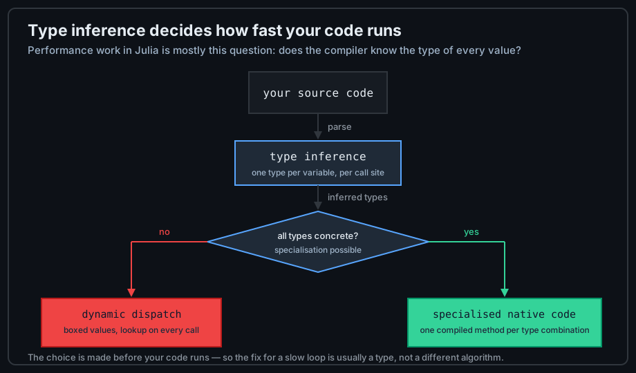
# Type-UNSTABLE: the return type depends on a value, not on the argument types
function pick_unstable(x)
    x > 0 ? 1 : 1.0                 # Int or Float64, chosen at run time
end

@code_warntype pick_unstable(1)      # Body::Union{Float64, Int64} — flagged

# Type-STABLE: one return type per argument type
pick_stable(x) = x > 0 ? 1.0 : 0.0
@code_warntype pick_stable(1)        # Body::Float64

# The same idea with containers: an element type inference cannot fix
function collect_unstable(v)
    out = []                         # Vector{Any}
    for x in v
        push!(out, x)
    end
    out
end

function collect_stable(v::AbstractVector{T}) where {T}
    out = Vector{T}(undef, 0)        # Vector{T}: concrete from the start
    for x in v
        push!(out, x)
    end
    out
end

@code_warntype collect_stable([1, 2, 3])    # Vector{Int64}

# Small unions are fine; a growing union is not
maybe_int(x) = x > 0 ? 1 : nothing          # Union{Int, Nothing} — acceptable
@code_warntype maybe_int(1)

# Reading the report:
#   red  = abstract or unknown type: the compiler gave up
#   blue = concrete type: fully specialised
# A stable function shows no red in its body.

Union returns are idiomatic at API boundaries — tryparse and findfirst both use them — but inside a hot loop they force the compiler to box each value. Keep the union at the edge and narrow it before the loop, as the next chapter shows.

Measuring Performance

Every performance claim needs a number, and every number needs a method. Julia's measurement story has three levels — a quick macro, a rigorous benchmark package, and a sampling profiler — and using the wrong level is itself a common source of wasted effort.

@time, @elapsed, and @allocated

The built-in macros are cheap and immediate, which makes them the right first probe. Their weakness is that a single measurement cannot separate compilation from execution, nor noise from signal.

# @time prints time, allocations, and GC time for ONE call
@time squaresum([1.0, 2.0, 3.0])      # includes compilation on the first call
@time squaresum([1.0, 2.0, 3.0])      # warm: the honest number

# @elapsed returns just the seconds — useful inside scripts
t = @elapsed sum(rand(1_000_000))
round(t * 1000, digits = 2)           # milliseconds

# @allocated returns bytes: the number that matters most inside loops
@allocated squaresum([1.0, 2.0, 3.0])         # 0 bytes — allocates nothing
@allocated apply_any(double, [1.0, 2.0])      # > 0 — boxing and vector growth

# Measure a block, not a single call
@time begin
    v = rand(1000)
    squaresum(v)
end

# The classic mistake: measure the compiler, then blame the code
@time squaresum(rand(1000))           # slow — first call with Vector{Float64}
@time squaresum(rand(1000))           # fast — same types, code already built

# Force compilation before measuring, then time many calls
squaresum(rand(1000))                 # deliberate warm-up
@time for _ in 1:10_000
    squaresum(rand(1000))             # rand allocates: time is dominated by it
end

Read @time output as three separate facts: total time, allocation count, and GC time. Heavy GC time says you are allocating; a large allocation count in a numeric loop almost always points at a type problem rather than an algorithmic one.

BenchmarkTools

@btime samples the expression many times, chooses a sensible number of evaluations, and reports a minimum, a median, and a spread. Interpolation with $ removes the cost of evaluating the arguments — otherwise you would be timing the setup rather than the code.

using BenchmarkTools

v = rand(1000)

# Interpolate the DATA, not the call: $v avoids timing a global lookup
@btime squaresum($v)                  # minimum time over many samples
@benchmark squaresum($v)              # the full statistics object

# Typical @btime output, read line by line:
#   1.230 μs (0 allocations: 0 bytes)
#     - the first number is the MINIMUM, not the mean
#     - the allocation count belongs to the whole expression
#     - a spread is printed when samples disagree badly

# Setup and teardown keep one-time work out of the measurement
@btime sort!(copy($v))                       # the copy is counted: honest cost
@btime sort!($x) setup = (x = copy($v))      # the copy is excluded

# Compare two implementations on the same data
slow_sum(v) = sum(x -> x^2, v)
fast_sum(v) = squaresum(v)

@btime slow_sum($v)                   # a closure applied per element
@btime fast_sum($v)                   # tight loop

# Relative comparison keeps the units readable
t1 = @belapsed slow_sum($v)
t2 = @belapsed fast_sum($v)
round(t1 / t2, digits = 2)            # e.g. 2.4 — the slowdown factor

Two rules make benchmark numbers trustworthy: interpolate everything that is not the code under test, and never benchmark at global scope. A bare global variable is a type-unstable access, so a naive benchmark measures the wrong thing entirely.

Profiling

A profiler answers a different question: not "how long does this call take" but "where did the time go". Sampling the program while it runs reveals hotspots you did not suspect, which is why profiling comes before optimising anything large.

using Profile

# Sample the program, then print a flat profile
@profile work()
Profile.print()                       # per-function sample counts

# Clear old samples between experiments
Profile.clear()

# Sample a short block at a higher rate
@profile begin
    for _ in 1:1000
        work()
    end
end

# Print only the heaviest entries, sorted by self time
Profile.print(format = :flat, sortedby = :count, mincount = 10)

# Inspect the compiled code for the suspected function
@code_warntype work()                 # types first — always start here
@code_llvm work()                     # optimised LLVM IR
@code_native work()                   # final assembly (look for vector ops)

# Tell-tale signs in the assembly
#   vaddpd / mulpd   → the float loop is vectorised (SIMD is happening)
#   callq ... jl_    → a call into the runtime: boxing or dynamic dispatch

The efficient order of operations is always the same: profile to find the hotspot, @code_warntype to explain it, make one change, then re-run the identical benchmark. Optimising a function that never appears in the profile is the most common way to spend a day for nothing.

Making Code Type-Stable

Almost every accidental slowdown traces back to one of three erasures of type information: a global variable, an abstractly typed container, or a variable that changes type inside a function. Each has a small, mechanical fix.

Global Variables and const

Code at the top level of a script is not compiled like a function. A non-constant global can change type between two calls, so the compiler refuses to assume anything and every read becomes a runtime lookup.

# BAD: a non-const global — the compiler cannot know its type
factor = 2.0
function scale_bad(v)
    out = similar(v)
    for i in eachindex(v)
        out[i] = v[i] * factor        # global read: type unstable
    end
    out
end

@code_warntype scale_bad([1.0, 2.0])  # red — factor is Any

# FIX 1: const, when the binding never changes type
const FACTOR = 2.0
function scale_const(v)
    out = similar(v)
    for i in eachindex(v)
        out[i] = v[i] * FACTOR        # constant folded: as fast as a literal
    end
    out
end

# FIX 2: pass it as an argument — the most flexible fix
scale_arg(v, k) = (out = similar(v); for i in eachindex(v); out[i] = v[i] * k; end; out)
scale_arg([1.0, 2.0], 2.0)

# FIX 3: when the type really is unknown, annotate the binding
x::Float64 = 2.0
function scale_typed(v)
    out = similar(v)
    for i in eachindex(v)
        out[i] = v[i] * x             # the assertion makes the read concrete
    end
    out
end

# FIX 4: wrap everything in a function — a common idiom for scripts
function main()
    factor = 2.0                      # a local, not a global
    scale_arg([1.0, 2.0], factor)
end
main()                                # this is the fast version

The const habit is worth adopting at file scope: constants cost nothing, document the value, and remove a whole class of inference failure. When the value must vary, pass it — arguments are always the cleanest channel for a type.

Abstract Element Types

A container's element type is a promise about every value it will ever hold. Declaring it abstractly — Vector{Any}, Vector{Real}, a struct field typed AbstractString — forces a pointer indirection and a boxed allocation for every element.

# BAD: an abstractly typed field and container
struct BadRow
    label::AbstractString             # abstract field type
    values::Vector{Real}              # abstract element type
end

# GOOD: parametrise the struct so the concrete types survive
struct GoodRow{S <: AbstractString, V <: AbstractVector}
    label::S
    values::V
end

row_bad = BadRow("a", Real[1, 2.5])
row_good = GoodRow("a", [1.0, 2.5])
typeof(row_good)                      # GoodRow{String, Vector{Float64}}

# Summing: the bad row boxes every element, the good row does not
total(r::BadRow) = sum(r.values)
total(r::GoodRow) = sum(r.values)

@code_warntype total(row_bad)         # Union — abstract
@code_warntype total(row_good)        # Float64 — concrete

# Same rule for function signatures: do not over-constrain
sum_any(v::Vector{Real}) = sum(v)             # accepts only Vector{Real} — rare
sum_abstract(v::AbstractVector{<:Real}) = sum(v)   # accepts Vector{Float64} etc.

sum_abstract([1.0, 2.0])                      # 3.0 — fast and general

# Parameters keep unrelated types apart, which avoids conversions
struct Pair2{A, B}
    first::A
    second::B
end
Pair2(1, "one")                       # Pair2{Int64, String}

Rules of thumb: never write Vector{Any} unless the elements genuinely differ in type; never put an abstract type in a struct field; and prefer a type parameter over an abstract annotation in method signatures. Each keeps element types known at compile time.

Function Barriers

When one piece of a function is unavoidably type-unstable, the instability must not spread. Putting the unstable code behind a function call — a "barrier" — confines it, because the barrier's argument and return types are still concrete.

# A value read from a file cannot be typed statically
function run_bad(spec::Dict)
    acc = 0
    for (k, v) in spec                 # v is Any: every use is unstable
        acc += v                       # boxing here...
    end
    acc
end

# BARRIER: the unstable part decides, the stable part computes
add_one(x::Int) = x + 1
add_one(x) = x                      # fallback for any other type

function run_good(spec::Dict)
    acc = 0
    for (k, v) in spec
        acc += add_one(v)              # ONE dynamic call per element, then stable
    end
    acc
end

# The barrier idea applies to loops over heterogeneous collections
mixed = Any[1, 2, 3]
typed = collect(Int, mixed)            # narrow once, at the boundary
squaresum(typed)                       # then run the fast path

# A closure that captures a reassigned variable becomes boxed —
# fix it by narrowing inside a let block or a helper function
function closure_bad(n)
    total = 0
    f = x -> (total += x)              # `total` is boxed: captured and reassigned
    for i in 1:n
        f(i)
    end
    total
end

function closure_good(n)
    f = let total = 0
        x -> total + x                 # read-only capture: no box
    end
    f(1)
end

Function barriers are the standard answer to "the data is dynamic but the work is numeric". Pay one dynamic dispatch at the boundary, then run compiled code inside — that is exactly the shape of @code_warntype-clean numeric kernels.

Allocations and Memory

Allocation is the second lever after types, and often the difference between 10× and 100×. Each allocation costs the allocator, the garbage collector, and the cache — and inside a loop, all three costs are multiplied by the iteration count.

Counting and Avoiding Allocations

The ! convention signals a function that writes into an argument instead of returning a new array. Combined with preallocation, it turns a loop that allocated once per iteration into a loop that allocates nothing.

# Allocating version: a new array on every call
add_allocating(a, b) = a .+ b
@allocated add_allocating(rand(1000), rand(1000))

# In-place version: the caller owns the output buffer
function add!(out, a, b)
    for i in eachindex(a, b, out)
        out[i] = a[i] + b[i]
    end
    out
end

out = zeros(1000)
@allocated add!(out, rand(1000), rand(1000))   # 0 bytes for the operation

# Preallocate once, reuse inside the loop
function sweep!(out, xs, ys)
    for k in eachindex(xs)
        add!(out, xs[k], ys[k])
    end
    out
end

# Accumulate in a variable, not in a growing vector
function mean_allocating(v)
    seen = []
    for x in v
        push!(seen, x)                 # the vector grows: repeated reallocation
    end
    sum(seen) / length(seen)
end

mean_better(v) = sum(v) / length(v)    # no intermediate storage at all

# When a growing collection is genuinely needed, size it first
function collect_if(cond, v, n)
    out = Vector{eltype(v)}(undef, 0)
    sizehint!(out, n)                  # reserve capacity: fewer reallocations
    for x in v
        cond(x) && push!(out, x)
    end
    out
end

collect_if(iseven, 1:10, 10)           # [2, 4, 6, 8, 10]

Measuring this is a two-line habit: wrap the candidate in @allocated before and after the change. A numeric kernel whose input and output are preallocated should report 0 bytes; anything else is a target.

Views and Broadcast Fusion

Slicing with a[1:10] copies; slicing with @view a[1:10] refers to the same memory. The dot syntax goes further: because . is part of the syntax, a .* b .+ c compiles to a single fused loop with no temporary arrays.

a = collect(1.0:100.0)

# Slicing copies — fine once, expensive inside a loop
row_copy = a[1:10]
@allocated a[1:10]                     # allocates 80 bytes

# A view refers to the original memory: no copy, no allocation
row_view = @view a[1:10]
@allocated @view a[1:10]               # 0 bytes

# Mutating through a view mutates the original
row_view[1] = 99.0
a[1]                                   # 99.0 — the same memory

# @views turns every slice in a block into a view
@views begin
    s = sum(a[5:15])                   # a view, not a copy
end

# Broadcast is fused: one loop, not two passes with an intermediate array
b = rand(100)
c = rand(100)
d = rand(100)
result = a[1:100] .* b .+ c .- d       # ONE loop over 100 elements
@allocated (a[1:100] .* b .+ c .- d)   # only the final result array

# In-place broadcasting writes into an existing buffer
dest = zeros(100)
dest .= b .+ c                         # no allocation at all
@allocated (dest .= b .+ c)            # 0 bytes

# Dot-fusion rule: .= for assignment, operands are arrays or scalars
dest .= sin.(b) .+ exp.(c)             # one fused loop

Two warnings. A view keeps its parent array alive, so a stored view also pins the whole array; and fusion happens only inside a single dotted expression — writing x = A .* B then y = x .+ C creates two loops and one intermediate.

Cache Locality and Struct Layout

After the type system and the allocator, the last large factor is memory order. Julia arrays are column-major and structs of plain bits are stored inline — both facts decide whether a loop streams through cache or scatters across it.

# Column-major: a column of a matrix is contiguous, a row is strided
M = rand(1000, 1000)

function sum_cols(M)
    s = 0.0
    for i in axes(M, 1), j in axes(M, 2)
        s += M[i, j]                   # inner loop walks a column: contiguous
    end
    s
end

function sum_rows(M)
    s = 0.0
    for j in axes(M, 2), i in axes(M, 1)
        s += M[i, j]                   # inner loop walks a row: strided
    end
    s
end

# Same result, different speed: benchmark both and see the gap
@btime sum_cols($M)                    # fast — sequential access
@btime sum_rows($M)                    # slower — cache-unfriendly access

# The same rule applies to element order: index the FASTEST axis innermost
v = zeros(1000)
for i in eachindex(v)                  # eachindex is a linear walk
    v[i] = 2i
end

# Struct layout matters too: keep hot data in compact isbits structs
struct Point                           # 16 bytes, stored inline in an array
    x::Float64
    y::Float64
end

struct PointAny                        # concrete fields, but boxed values
    x::Any
    y::Any
end

isbitstype(Point)                      # true — values live inline
isbitstype(PointAny)                   # false — every field is a heap reference

points = [Point(rand(), rand()) for _ in 1:1000]   # one contiguous block
@allocated points                                   # a single allocation

# @simd lets the compiler reorder independent iterations
function fast_sum(v)
    s = 0.0
    @simd for x in v
        s += x                         # iterations independent: reordering is safe
    end
    s
end

Choose the loop order that matches the storage order, keep hot data in isbits structs, and use @simd only when the iterations are genuinely independent. These are the changes that move a numeric kernel from memory-bound towards compute-bound.

The Optimisation Workflow

Optimisation is a procedure, not a bag of tricks. Following it in order keeps you from rewriting code that was never the problem — and from shipping an unsafe shortcut that buys nothing.

Measure, Don't Guess

The first rule is to find the real cost centre before touching anything. Intuition about which line is slow is wrong often enough that experienced engineers still profile first.

# 1. Establish a baseline with a realistic input
data = rand(10_000_000)

function pipeline(data)
    a = data .* 2.0                  # allocation per call
    b = filter(x -> x > 1.0, a)      # another allocation
    sum(b)                           # a reduction
end

@btime pipeline($data)               # the number you must beat

# 2. Profile to locate the hotspot
using Profile
@profile pipeline(data)
Profile.print(format = :flat, sortedby = :count)

# 3. Make ONE change and re-measure the SAME benchmark
function pipeline_fused(data)
    s = 0.0
    @inbounds for x in data
        y = 2x
        y > 1.0 && (s += y)         # fused: no intermediate arrays
    end
    s
end

@btime pipeline_fused($data)         # compare against the baseline

# 4. Record the change and the numbers so the next person can repeat it
#    baseline: 42 ms · after fusion: 9 ms · input: 10^7 Float64

# Amdahl's law in one line: if a step is 10% of the time, perfecting it
# gives at most a 10% speedup. Find the 90% first.

Keep the benchmark beside the code while iterating, and change one thing at a time. A speedup you cannot attribute to a single change is a speedup you cannot defend later.

Escape Hatches and Their Cost

When the safe version is already clean — stable types, no allocations — the remaining gains come from switches that disable a safety check. Each has a condition you must prove yourself, because the compiler will no longer check it for you.

# @inbounds removes bounds checks: prove the indices are valid
function unsafe_sum(v)
    s = 0.0
    @inbounds for i in eachindex(v)   # eachindex already guarantees validity
        s += v[i]
    end
    s
end

# WRONG: a hand-written index that can exceed the array
function broken(v)
    s = 0.0
    @inbounds for i in 1:length(v) + 1
        s += v[i]                      # reads past the end: undefined behaviour
    end
    s
end

# @fastmath allows reassociation: only for float code that tolerates it
@fastmath sum(sin.(rand(1000)))        # may differ in the last bits

# unsafe_wrap borrows raw memory — useful with C, dangerous with GC
using Base: unsafe_wrap
raw = [1.0, 2.0, 3.0]
wrapped = unsafe_wrap(Array, pointer(raw), 3)   # views the same memory

# GC.@preserve keeps an object alive while a pointer to it is in use
function hash_first(v)
    GC.@preserve v begin
        p = pointer(v)
        unsafe_load(p)
    end
end

# The order to reach for them:
#   1. fix types
#   2. remove allocations
#   3. reorder loops / fuse broadcasts
#   4. @inbounds and @simd, guarded by eachindex
#   5. @fastmath or unsafe only with a benchmark that justifies it

An escape hatch that produces a 3% gain is a bad trade against a crash you will debug at 3 a.m. Keep the safe code commented next to the unsafe version, and keep a test that exercises the boundary — the first and last element, and an empty input.

Startup, Compilation, and Memory

Interactive speed and production speed are different problems. A script that starts in ten seconds because it compiles on the fly is perfectly fast in a notebook and unacceptable behind an HTTP endpoint, so production needs its own set of decisions.

# Measure time to first result, not throughput
julia --startup-file=no script.jl                # baseline: includes compilation

# Julia 1.9+ caches compiled code in a package's pkgimage automatically;
# for a script, move the hot code into a package or use PrecompileTools
using PrecompileTools
@setup_workload begin
    @compile_workload begin
        squaresum([1.0, 2.0, 3.0])               # precompiled into the cache
        pipeline_fused(rand(100))
    end
end

# A system image bakes the whole dependency graph into one binary
#   julia> using PackageCompiler
#   julia> create_sysimage([:MyPkg]; sysimage_path = "my.so")

# Memory: report what the process actually holds
Base.gc_live_bytes()             # bytes currently live
@time Base.GC.gc(true)           # force a collection and see the cost

# Reduce peak memory by streaming instead of materialising
function stream_sum(path)
    s = 0.0
    open(path) do io
        for line in eachline(io)
            s += parse(Float64, line)            # one line in memory at a time
        end
    end
    s
end

Three production levers, in order of effect: precompile the workload a request will hit, keep allocations out of the request path, and stream large data instead of loading it. Only after those does a system image become worth its build complexity.

Common Pitfalls

Performance mistakes in Julia cluster into a few recognisable shapes. Naming them is usually enough to stop repeating them.

Benchmarking the First Call

The first call to a method with a new type combination includes compilation, so it can be thousands of times slower than every later call. A benchmark that measures it once reports the compiler's speed, not your code's.

# WRONG: one call, cold — the number is almost entirely compilation
@time heavy_analysis(rand(100))

# WRONG even with @btime if the arguments are freshly evaluated globals
@btime heavy_analysis(rand(100))       # rand(100) is inside the timing!
@btime heavy_analysis($(rand(100)))    # data created once, outside the loop

# RIGHT: warm up, then measure with interpolated data
heavy_analysis(rand(100))              # compile for Vector{Float64}
data = rand(100)
@btime heavy_analysis($data)           # time the code, not rand or the compiler

# Watch for the same trap inside setup blocks
@btime solve($x) setup = (x = build_model())   # build_model is compiled too —
                                               # run it once before the benchmark

# A quick sanity check on any number: run the benchmark twice.
# If the second run is much faster, you measured compilation.
@btime warm_path($data)
@btime warm_path($data)

Two habits remove this entire class of error: always warm the exact type combination you intend to measure, and always interpolate inputs so the benchmark measures only the expression you care about.

Optimising the Wrong Thing

A 20% improvement to a function that consumes 2% of the runtime changes nothing measurable. Without a profile, "obvious" hotspots are frequently not hotspots at all.

# Two helpers, one hot — but which?
parse_row(line) = split(line, ',')            # looks cheap
compute(row) = sum(parse(Float64, x) for x in row)   # looks expensive

function load(csv_lines)
    total = 0.0
    for line in csv_lines
        total += compute(parse_row(line))
    end
    total
end

# The profile decides — do not argue with the data
using Profile
@profile load(lines)
Profile.print(format = :flat, sortedby = :count)

# Only then optimise the function that owns the samples
# Example outcome: 78% in compute, 3% in parse_row
#   → optimising parse_row (even to zero cost) can give at most 3%

# Re-measure after each change, with the same input size
@btime load($lines)

Amdahl's law is the reason: the ceiling on your total gain is set by the fraction of time the changed code consumes. Optimising the 3% is a hobby; optimising the 78% is engineering.

Type Instability by Habit

The fourth category is not a mistake in a single line but a habit carried over from dynamic languages — starting from [], returning different types from branches, or storing heterogeneous values in one field.

# HABIT 1: an untyped empty vector
bad1() = (out = []; push!(out, 1); out)              # Vector{Any}
good1() = (out = Int[]; push!(out, 1); out)          # Vector{Int64}

# HABIT 2: branches returning different concrete types
bad2(x) = x > 0 ? x : "none"                         # Union{Int64, String}
good2(x) = x > 0 ? string(x) : "none"                # always String

# HABIT 3: a heterogeneous dictionary used in a hot path
config = Dict{String, Any}("n" => 10, "tol" => 1e-9)
# fix: type the values, or convert once at the boundary
n = config["n"]::Int

# HABIT 4: an abstract field in a struct used in a loop
struct Box
    v::Any
end
# fix: parametrise
struct BoxT{T}
    v::T
end

# Check the habits with one command per function
@code_warntype good1()
@code_warntype good2(1)
@code_warntype BoxT(1)

# And a tidy summary of inference for a whole call
@inferred sum_abstract([1.0, 2.0])     # passes only if the type is concrete
@inferred squaresum([1.0, 2.0])

Treat @code_warntype and @inferred as tests: run them on the functions on your hot path and fix every red type. It is a five-minute check that prevents most of the slowdowns in this lesson.

Every lever in this lesson applies to a single thread. The next step is using more than one: Parallelism & Async covers tasks, threads, and channels — and the new kinds of bug that appear once two pieces of code run at the same time.