Data-Oriented Design (SOA/AOS)

Nothing here is Odin-specific. C, C++, C#, and Rust programmers have all discovered the same thing, and the same diagram explains all of them. What makes Odin unusual is that the language gives you direct, readable support for the layout that wins.

Why Layout Beats Cleverness

Let us start with the uncomfortable fact that motivates the whole subject.

The Memory Wall

Processors got fast; memory did not get fast at the same rate. The result is that a value the processor needs might cost a few cycles if it is already nearby, and a couple of hundred cycles if it has to come from main memory. In a tight loop, almost all the time goes into waiting for data, not computing with it.

Hardware compensates with caches: small, fast memories that hold recently used data. And it fills those caches in fixed-size blocks rather than one value at a time. Which brings us to the single most useful number in performance work.

Cache Lines, Not Elements

Memory is moved in cache lines, and on the usual 64-bit processors a line is 64 bytes. When your code touches one byte, the processor fetches 64. That is a bargain if you were about to use the other 63, and a waste if you were not.

Read that again, because the whole lesson follows from it: you are never charged for one value; you are charged for a block of them. Two programs with identical algorithms can differ by several times in speed depending on whether they use the bytes they paid for.

Array of Structs (the Default)

The layout you get for free is the one you would write down naturally: define a record, then make an array of them.

Records Stored Whole

Vector2 :: [2]f32           // two floats = 8 bytes, with array arithmetic

Particle :: struct {
    position: Vector2,      // 8 bytes
    velocity: Vector2,      // 8 bytes
    mass:     f32,          // 4 bytes
    health:   f32,          // 4 bytes
}

#assert(size_of(Particle) == 24)   // 24 bytes per particle, with no padding

// A normal slice stores the records whole: AOS — array of structs.
particles := make([]Particle, count)
defer delete(particles)

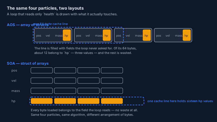
In memory, a slice of these looks like a row of identical boxes: position velocity mass health, then position velocity mass health, and so on. That is what "array of structs" means, and it is a perfectly reasonable layout — especially when a piece of code needs all the fields of one record at a time.

What You Pay For

The trouble starts when a loop needs only some of the fields. Here is the least flattering case — a regeneration pass that touches nothing but health:

dt: f32 = 1.0 / 60.0
regen: f32 = 2.0

// This loop uses 4 bytes out of every 24 that are loaded.
for i in 0..<len(particles) {
    particles[i].health += regen * dt
}

Follow what the hardware does. The first particle's health is somewhere inside a 24-byte record, so the processor fetches the whole cache line containing it — three or four records' worth of bytes. The loop then reads four useful bytes and steps to the next record, which is very likely inside that same line. So for every line loaded from memory, the loop uses perhaps 12 or 16 bytes out of 64 and discards the rest.

A movement pass does better, because it uses two fields instead of one:

// 16 useful bytes out of each 24 — better, but still a third wasted.
for i in 0..<len(particles) {
    particles[i].position += particles[i].velocity * dt
}

The pattern to notice: the more fields a loop ignores, the more of the line it throws away. And a game, a simulation, or a data pipeline is normally full of narrow loops — physics here, health there, rendering somewhere else. Each one pays for the fields it never reads.

Struct of Arrays

The remedy is almost embarrassingly simple: stop storing the records whole. Keep one array per field, so that the values a loop needs are the only values in the lines it loads.

One Array Per Field

// The same particles, split by field: each field becomes a contiguous array.
positions  := make([]Vector2, count)
velocities := make([]Vector2, count)
healths    := make([]f32,     count)
// (and masses, omitted here for brevity)

// Freeing is per slice, exactly as before.
defer delete(positions)
defer delete(velocities)
defer delete(healths)

Now the regeneration pass reads one array and nothing else:

// Every byte of every line loaded belongs to `healths`.
for i in 0..<len(healths) {
    healths[i] += regen * dt
}

The Loop That Wins

Compare the two versions of that loop honestly. Same operation, same result, same number of iterations. The only difference is which bytes sit next to each other in memory.

• AOS: the loop fetches a 64-byte cache line, and gets two or three health values out of it before the line is exhausted.
• SOA: the same 64-byte line holds sixteen consecutive health values — all of them useful, none of them thrown away.

And the code that needs several fields still works; it simply indexes each array at the same position:

// A loop that needs two fields reads from two arrays.
for i in 0..<len(positions) {
    positions[i] += velocities[i] * dt
}

That is the whole trade, stated plainly: SOA makes narrow loops fast and wide loops slightly more verbose. Simulation and game code is full of narrow loops, which is why the trade usually wins there — and why a straightforward business application should probably keep its readable structs and not think about this at all.

SOA in Odin

Splitting data by hand is tedious and easy to get subtly wrong: one array per field to keep in step, and one delete per array. Odin lets you ask for the split layout directly.

The #soa Type

Write #soa in front of the array type, and the storage becomes struct-of-arrays while the element type stays exactly what you wrote:

Particle :: struct {
    position: Vector2,
    velocity: Vector2,
    mass:     f32,
    health:   f32,
}

// A normal slice: records stored whole (AOS).
whole: []Particle

// A SOA slice: the SAME element type, stored field by field.
split: #soa[]Particle

Both are slices of Particle. The difference is entirely in the arrangement of the bytes — and a loop that reads one field benefits from the second in exactly the way the hand-split version did, except that you wrote one type instead of four arrays.

// The same idea is available for the other array shapes:
fixed:   #soa[1024]Particle      // a fixed count, known at compile time
growing: #soa[dynamic]Particle   // grows like a dynamic array

Odin's own type information treats this as a layout rather than a new kind of data: it records whether a struct is stored plain, or in one of three SOA forms — fixed, slice, or dynamic. One struct, four possible arrangements, chosen where you declare it.

soa_zip and soa_unzip

Often the data already lives in separate arrays, because that is how it arrived or how another part of the system prefers it. Two built-ins convert between the views in one call. Here are their signatures, quoted exactly as the language declares them:

soa_zip   :: proc(slices: ...) -> #soa[]Struct
soa_unzip :: proc(value: $S/#soa[]$E) -> (slices: ...)

soa_zip takes several field slices and presents them as one SOA array; soa_unzip hands the field slices back. That is what makes the style practical in a real program: your hot loop sees the layout it wants, and the rest of the code keeps working field by field without knowing that anything changed.

Measuring Instead of Believing

The layout argument is easy to accept and just as easy to over-apply. A loop that runs a hundred times will not care about cache lines, and making it less readable buys nothing. So the professional habit is to measure.

Timing Your Own Code

Odin gives you two useful sources of time. For most comparisons, wall-clock time is enough:

import "core:time"

// Take a time, run the work, take another time, subtract.
start := time.now()

for i in 0..<len(healths) {
    healths[i] += regen * dt
}

elapsed := time.since(start)
fmt.println("elapsed:", elapsed)

For finer work there is the processor's own cycle counter, read_cycle_counter(), which counts cycles rather than seconds — the right unit when you are comparing two loops that each take microseconds. Check core:time for the exact helpers available in your release; the shape of every measurement is the one above: take a time, do the work, take another, subtract.

When It Is Worth It

• Many elements, one operation. Layout pays off in loops over thousands of items and is irrelevant for ten.
• A narrow hot loop. A loop that reads a fraction of each record is the signature case. If a loop touches every field, AOS is fine and simpler.
• Measure, change, measure. Guessing which loop is hot is famously unreliable, and it is easy to make a cold loop uglier for no gain at all.
• Leave the rest of the program alone. Business logic over a few hundred records should stay readable. Data-oriented design is a tool for the part of the program that runs a million times.

Bits: Layout at the Smallest Scale

Before leaving memory and layout behind, there is one more scale to look at — the smallest one. The set type used in this track is called a bit set for a reason, and the reason is worth seeing once.

The Storage Behind a bit_set

Back in the operators lesson you packed flags into a u8 by hand. Here is that same picture again, thought of as storage rather than as arithmetic:

// Eight yes/no facts — permissions, options, flags — fit in one byte.
Read    :: 0b0000_0001
Write   :: 0b0000_0010
Execute :: 0b0000_0100

// A byte holding "Read and Write" looks like this:
mine: u8 = Read | Write           // 0b0000_0011

fmt.println("mine:", mine)            // 3 — as a number
fmt.printf("mine: %b\n", mine)        // 11 — as bits, which is the real layout

Printing a value in binary is the fastest way to see a layout. The number 3 tells you very little; 11 tells you that two switches are on, and which two.

Now the important part. The three operations from that lesson are not arbitrary — they are the three operations every set needs, expressed on the storage:

Nothing about that table is specific to Odin; it is what a bit pattern is. Which is also why the next step is so short.

What That Means for the Set Type

Odin's bit_set is exactly this storage, with names on the bits and a syntax that reads like English. When you write .Read in permissions, the machine is testing one bit. When you add a member with +, it is setting one. The set never becomes a data structure with a pointer and an allocation — it is the bits, which is why it costs nothing to create and nothing to free.

Two minutes at a keyboard will teach you the remaining operators better than any table. Print two sets, apply each bitwise operator, and read what comes back:

Permission  :: enum { Read, Write, Execute }
Permissions :: bit_set[Permission]

read_write: Permissions = { .Read, .Write }
write_exec: Permissions = { .Write, .Execute }

fmt.println(read_write)     // Permissions{Read, Write}
fmt.println(write_exec)     // Permissions{Write, Execute}

// Now try & and | and &~ between the two, and watch the members change.

That is the honest way to learn a representation: look at the storage, change it, and check your understanding against what appears. It is also the habit that makes the rest of this track easier, because every performance idea you meet from here on is ultimately a statement about bytes.

Where This Goes Next

Phase 4 is complete, and with it the half of the track that deals with the machine. Phase 5 is about the other half of reliability: how Odin reports failure — with errors as values, defer for cleanup, and or_return to pass a failure along without hiding it.

The Page in One Breath

• Memory moves in cache lines — 64 bytes on the usual 64-bit processors — so a loop pays for a block whether or not it uses all of it.
• AOS stores records whole: natural to write, wasteful for narrow loops.
• SOA stores one array per field, so the lines a narrow loop loads are entirely made of the field it wants.
• Same algorithm, same results — only the arrangement of bytes changes.
• Odin writes the split layout as a type: #soa[]T, #soa[N]T, or #soa[dynamic]T.
• soa_zip and soa_unzip convert between separate field slices and an SOA array.
• Measure before and after: core:time for seconds, the cycle counter for cycles.
• A bit set is that same storage at the smallest scale — the bitwise operators on its bits are the set operations.
• Do not apply this everywhere — reach for it in the loop that runs a million times.

Continue with Errors, defer & or_return — the beginning of Phase 5 →