
Shortest Paths & Minimum Spanning Trees
The Shortest-Path Problem
Given a weighted graph and a source vertex, find the minimum total weight to every other vertex, together with the routes. Every algorithm in this section is built on a single operation.
Relaxation
Keep a tentative distance dist[v] for every vertex, starting at infinity (0 for the source). Relaxing an edge u → v with weight w asks whether going through u gives a shorter route to v:
if dist[u] + w < dist[v] {
	dist[v] = dist[u] + w
	prev[v] = u // remember the route, as parent[] did in BFS
}
The algorithms differ only in the order in which they relax edges and in how many times they relax each one. That order determines both their speed and which graphs they handle correctly.
Choosing an Algorithm
| Graph | Algorithm | Time |
|---|---|---|
| unweighted (all weights equal) | BFS (Graph Traversal) | O(V + E) |
| DAG, any weights | relax in topological order | O(V + E) |
| non-negative weights | Dijkstra | O((V + E) log V) |
| one target and a good distance estimate | A* | often far less than Dijkstra |
| negative weights | Bellman-Ford | O(V · E) |
| all pairs, small V | Floyd-Warshall | O(V³) |
Dijkstra's Algorithm
Dijkstra generalizes BFS by replacing the FIFO queue with a priority queue keyed on distance. It always takes the unfinished vertex with the smallest tentative distance. That distance is then final: any other route would have to leave the finished region through a vertex that is at least as far away, and with non-negative weights the route cannot get shorter afterwards. Demo with route reconstruction, an all-pairs oracle check, and a million-edge graph: 42_dijkstra.go.
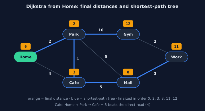
Final distances from Home (orange) and the shortest-path tree (blue). The direct road to the Cafe costs 4, but the route through the Park costs 3.
Dijkstra with container/heap
Updating a distance inside the heap requires the item's index and heap.Fix (see Heaps). The simpler and common alternative is lazy deletion: push a new entry whenever a distance improves, and skip entries for vertices that are already finished. The heap then holds at most E entries.
func dijkstra(adj [][]Edge, src int) (dist, prev []int, pops int) {
	n := len(adj)
	dist = make([]int, n)
	prev = make([]int, n)
	for i := range dist {
		dist[i], prev[i] = inf, -1
	}
	done := make([]bool, n) // done[v]: dist[v] is final
	dist[src] = 0
	h := &minHeap{{src, 0}}
	for h.Len() > 0 {
		cur := heap.Pop(h).(item)
		pops++
		if done[cur.v] {
			continue // stale entry: v is already final
		}
		done[cur.v] = true
		for _, e := range adj[cur.v] {
			if nd := cur.dist + e.w; nd < dist[e.to] {
				dist[e.to] = nd
				prev[e.to] = cur.v
				heap.Push(h, item{e.to, nd})
			}
		}
	}
	return dist, prev, pops
}
Every edge causes at most one push and every push one pop, each O(log E) = O(log V), so the total is O((V + E) log V). If you need only one target, stop when it is popped.
Why Negative Weights Break It
Dijkstra's correctness argument assumes that extending a path never makes it shorter. With a negative edge, a vertex that was already finalized can later be reached more cheaply. In the demo's four-vertex example, Dijkstra reports a distance of 3 where the true shortest distance is 2, and it reports no error. Negative weights appear with refunds, energy regained going downhill, and logarithms of exchange rates. They need the next algorithm.
Bellman-Ford and Negative Cycles
Bellman-Ford makes no assumptions: it relaxes every edge, V − 1 times. A shortest path without cycles has at most V − 1 edges, and after round k every shortest path of k edges has been found. Demo with negative-cycle extraction, an arbitrage detector, and a Floyd-Warshall oracle: 43_bellman_ford.go.
The Algorithm
for round := 1; round <= n; round++ {
	rounds = round
	changed := -1
	for _, e := range edges {
		if dist[e.from] != inf && dist[e.from]+e.w < dist[e.to]-1e-9 {
			dist[e.to] = dist[e.from] + e.w
			prev[e.to] = e.from
			changed = e.to
		}
	}
	if changed == -1 {
		return // nothing improved: all distances are final
	}
	if round == n {
		cycleAt = changed // still improving in round V: negative cycle
	}
}
The cost is O(V · E), much slower than Dijkstra on large graphs, but it is simple and general, and it often exits early: the demo's delivery graph settles after 3 rounds instead of the maximum 5. The small tolerance 1e-9 is needed only because the arbitrage example uses floating-point weights.
Detecting a Negative Cycle
If a loop's weights sum to less than zero, going around it again always lowers the cost, so "shortest path" has no answer. Bellman-Ford detects this: if a V-th round still improves some distance, a negative cycle can be reached from the source. Following prev links V times from that vertex is guaranteed to land on the cycle, and then you can walk it.
Example: Currency Arbitrage
Trading money along a cycle of currencies multiplies the exchange rates, and a profit means the product is greater than 1. Logarithms turn products into sums: product > 1 exactly when the sum of −log(rate) is below 0. With edge weights −log(rate), an arbitrage opportunity is a negative cycle. The demo finds USD → EUR → GBP → USD, which turns 1 unit into 1.0048 units.
All Pairs: Floyd-Warshall
For the distance between every pair of vertices in a small graph, Floyd-Warshall uses three nested loops. The outer loop allows each vertex k in turn as an intermediate stop. It runs in O(V³) time and O(V²) memory, which is practical up to a few thousand vertices. Its code is so short that it is easy to get right, which is why the demos use it as the oracle for Dijkstra and Bellman-Ford:
for k := range n {
	for i := range n {
		for j := range n {
			if d[i][k] != inf && d[k][j] != inf && d[i][k]+d[k][j] < d[i][j] {
				d[i][j] = d[i][k] + d[k][j]
			}
		}
	}
}
A* Search
Dijkstra grows a circle around the source in every direction. When there is a single target and you can estimate the remaining distance to it, A* searches toward the goal instead. It is the standard pathfinding algorithm in games, robotics, and route planners. Demo on a grid with a wall, drawn cell by cell, plus random mazes checked against BFS: 44_astar.go.
Ordering by g + h
A* orders its priority queue by f(v) = g(v) + h(v), where g is the known distance from the start and h is a heuristic estimate of the distance left. Everything else is Dijkstra's code. With h = 0, A* is Dijkstra; with a perfect h, it walks straight along the optimal path.
ng := cur.g + 1
if old, seen := g[n]; !seen || ng < old {
	g[n] = ng
	parent[n] = cur.p
	heap.Push(q, entry{n, ng + h(n), ng}) // priority f = g + h
}
Admissible Heuristics
A heuristic is admissible if it never overestimates the true remaining distance. With an admissible heuristic, A* still returns an optimal path. On a 4-connected grid with unit steps, the Manhattan distance |Δrow| + |Δcol| is admissible, because no route can be shorter than it. On a road map, the straight-line distance is admissible. In the demo, A* finds the same 36-step path as Dijkstra while expanding 87 cells instead of 231. Across 300 random mazes, it expands just over a third as many cells in total.
Trading Optimality for Speed
Multiplying the heuristic by a factor greater than 1 (weighted A*) makes the search greedier: it expands fewer cells but may return a longer path. Games often accept a slightly worse path for a faster answer. The demo shows the effect with 3 × Manhattan.
Minimum Spanning Trees
A spanning tree connects all V vertices of a connected, undirected graph with exactly V − 1 edges and no cycle. A minimum spanning tree (MST) has the smallest total weight: the cheapest way to lay cable to every building or connect every network node. Note that it minimizes the total weight; it is not a shortest-path tree. Demo with both algorithms checked against brute force: 45_minimum_spanning_tree.go.
The Cut Property
Split the vertices into any two groups. The lightest edge that crosses between them belongs to some MST: if an MST did not use it, adding it to that tree would create a cycle, the cycle would have to cross the split again through some other edge at least as heavy, and removing that edge would give a spanning tree that is no heavier. This one fact justifies both algorithms below, which are greedy: they commit to the locally cheapest safe edge and never reconsider. Phase 4 studies when greedy choices are correct in general.
Kruskal: Sort Edges, Skip Cycles
Sort all edges by weight and add each one unless it would close a cycle. Union-find from the previous lesson answers the cycle question in nearly O(1). The total cost is dominated by the sort: O(E log E).
func kruskal(n int, edges []Edge) (tree []Edge, total int, ok bool) {
	sorted := slices.Clone(edges)
	slices.SortFunc(sorted, func(a, b Edge) int { return cmp.Compare(a.w, b.w) })
	d := NewDSU(n)
	for _, e := range sorted {
		if d.Union(e.u, e.v) { // endpoints in different trees: no cycle
			tree = append(tree, e)
			total += e.w
			if len(tree) == n-1 {
				break // a spanning tree is complete
			}
		}
	}
	return tree, total, len(tree) == n-1
}
Prim: Grow One Tree
Start from any vertex and repeatedly add the lightest edge that leaves the current tree. The cut property applies with the split "in the tree" versus "not yet in the tree". A heap of candidate edges with lazy deletion, the same pattern as Dijkstra, gives O(E log V). Prim suits adjacency lists and dense graphs; Kruskal suits edge lists. The demo builds both MSTs of a complete graph on 2,000 random points (about two million edges) and gets identical total weights.
Common Pitfalls
Weighted graph bugs often produce plausible numbers, so check against a slow oracle.
Dijkstra on Negative Weights
It returns wrong distances silently. If any weight can be negative, use Bellman-Ford, or reweight the edges first (Johnson's algorithm).
Infinity Overflow
Using math.MaxInt as infinity and then computing dist[u] + w overflows to a large negative number, which looks like a very short path. Check for infinity before adding, as the Floyd-Warshall loop does, or use a sentinel far below the overflow limit.
MST on a Directed or Disconnected Graph
Kruskal and Prim assume an undirected graph. On a disconnected graph they return a minimum spanning forest with fewer than V − 1 edges; check the edge count, as the demo's ok result does. Directed graphs need a different algorithm (minimum arborescence).
Practice Lab
For each exercise, decide what the weights mean and whether any can be negative before you pick an algorithm.
Run the Demos
- In 42_dijkstra.go, turn the min-heap into a max-heap (
>inLess). How many random graphs disagree with Floyd-Warshall? - In 43_bellman_ford.go, run only V − 1 rounds (
round < n). Which checks fail, and why is the V-th round needed? - In 44_astar.go, use
3 * h(p)in the random-maze check. How many path lengths now differ from BFS? - In 45_minimum_spanning_tree.go, sort the edges in descending order in
kruskal. What do you get instead of an MST?
Exercises
- Network delay. Given directed travel times from a server, find how long a broadcast takes to reach every node, or report that some node is unreachable.
- Cheapest flight with at most k stops. Why does plain Dijkstra fail here? Adapt Bellman-Ford to run exactly k + 1 rounds.
- Path with maximum probability. Edges carry success probabilities. Find the most reliable route by adapting Dijkstra to multiply probabilities and prefer larger values.
- Connect all points. Given 2D points, connect them all with minimum total Manhattan distance. Compare Prim on the implicit complete graph with Kruskal on an explicit edge list.
Phase 3 is complete. Continue with Greedy Algorithms, the first lesson of Phase 4.