
Sorting
slices.Sort is excellent, so you will rarely write a sort in production. You study sorting because it teaches the core design strategies (incremental, divide and conquer, randomization, and using keys as indices) and the vocabulary for describing any algorithm: stable, in place, adaptive, worst case, and average case.
Describing a Sort
Every sorting algorithm is described along the same dimensions. They matter more than raw speed when choosing one.
Stable, In Place, Adaptive
- Stable: elements with equal keys keep their original relative order. This matters when sorting records by one field after another.
- In place: needs only O(1) or O(log n) extra memory.
- Adaptive: runs faster when the input is already nearly sorted.
| Algorithm | Best | Average | Worst | Memory | Stable |
|---|---|---|---|---|---|
| Insertion sort | O(n) | O(n²) | O(n²) | O(1) | yes |
| Selection sort | O(n²) | O(n²) | O(n²) | O(1) | no |
| Merge sort | O(n log n) | O(n log n) | O(n log n) | O(n) | yes |
| Quicksort (random pivot) | O(n log n) | O(n log n) | O(n²) | O(log n) | no |
| Heapsort (Heaps) | O(n log n) | O(n log n) | O(n log n) | O(1) | no |
| Counting sort | O(n + k) | O(n + k) | O(n + k) | O(n + k) | yes |
| Radix sort (d digits) | O(d(n + b)) | O(d(n + b)) | O(d(n + b)) | O(n + b) | yes |
The n log n Lower Bound
Any sort that learns about the data only by comparing elements needs about n log₂ n comparisons in the worst case. There are n! possible orderings of the input, and each comparison answers one yes-or-no question, so at least log₂(n!) ≈ n log₂ n answers are needed to tell them all apart. Merge sort and heapsort meet this bound, so no comparison sort can be asymptotically faster. Counting and radix sort get around it by not comparing at all.
Elementary Sorts
The O(n²) sorts are too slow for large inputs, but they are the right place to practise loop invariants. Insertion sort also appears inside every fast production sort. Demo that counts comparisons and moves and shows stability: 32_elementary_sorts.go.
Insertion Sort
Insertion sort works like sorting a hand of cards: take the next card and shift larger cards right until its place opens up. Invariant: at the start of each outer iteration, a[:i] is sorted.
func insertionSort(a []int, c *Counter) {
	for i := 1; i < len(a); i++ {
		x := a[i] // the card being inserted
		j := i - 1
		for j >= 0 {
			c.cmp++
			if a[j] <= x { // <= stops at equal keys: stable
				break
			}
			a[j+1] = a[j] // shift the larger element one step right
			c.moves++
			j--
		}
		a[j+1] = x
		c.moves++
	}
}
On sorted input the inner loop stops immediately, giving n − 1 comparisons in total. On reversed input every element travels to the front, giving n(n − 1)/2. The work equals the number of inversions (out-of-order pairs), which is why insertion sort is fast on nearly sorted data. Go's slices.Sort switches to insertion sort for ranges of 12 elements or fewer.
Selection and Bubble Sort
Selection sort finds the minimum of the unsorted part and swaps it to the front. It always makes n(n − 1)/2 comparisons but at most n − 1 swaps, which helps only when writes are very expensive. The long-distance swap can jump an element over an equal one, so it is not stable. Bubble sort swaps adjacent out-of-order pairs; with an early exit when a pass makes no swap, it is adaptive, but it moves elements one step at a time and is the slowest of the three in practice.
The demo sorts cards that have equal ranks. Insertion sort keeps 5a before 5b; selection sort outputs 5b before 5a.
Merge Sort
Merge sort is the standard example of divide and conquer: split the problem in half, solve each half recursively, and combine the results. Full demo with a recursion trace, a bottom-up version, and inversion counting: 33_merge_sort.go.
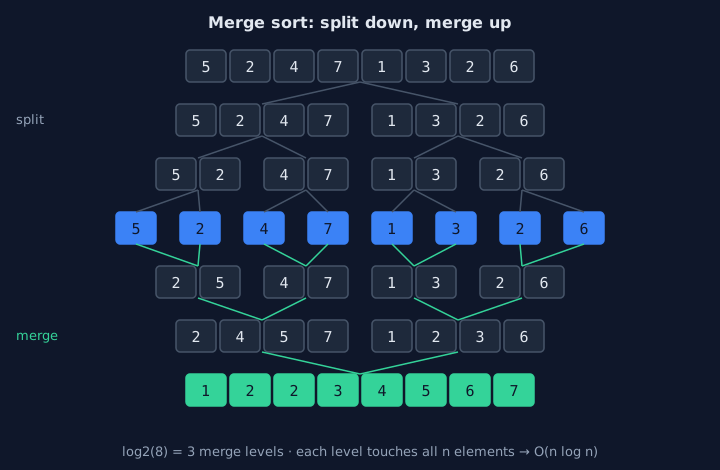
Splitting does no comparisons. All the work happens in the merges, where each of the log₂ n levels processes every element once.
The Merge Step
Two sorted halves are merged by repeatedly taking the smaller front element. Taking from the left half on ties is what makes merge sort stable.
// merge combines sorted a[lo:mid] and a[mid:hi] using buf as scratch space.
func merge(a, buf []int, lo, mid, hi int) {
	copy(buf[lo:hi], a[lo:hi])
	i, j := lo, mid // next unread element of each half
	for k := lo; k < hi; k++ {
		switch {
		case i == mid: // left half used up
			a[k] = buf[j]
			j++
		case j == hi: // right half used up
			a[k] = buf[i]
			i++
		case buf[j] < buf[i]: // strictly smaller: ties go left -> stable
			a[k] = buf[j]
			j++
		default:
			a[k] = buf[i]
			i++
		}
	}
}
Recursion and Cost
The recursion allocates one scratch buffer and shares it across all calls. If the last element of the left half is already no larger than the first element of the right half, the halves are in order and the merge can be skipped, which makes merge sort O(n) on sorted input.
sort = func(lo, hi int) {
	if hi-lo < 2 {
		return // 0 or 1 elements: already sorted (base case)
	}
	mid := lo + (hi-lo)/2
	sort(lo, mid)
	sort(mid, hi)
	if a[mid-1] <= a[mid] {
		return // halves already in order: skip the merge (O(n) on sorted input)
	}
	merge(a, buf, lo, mid, hi)
}
The cost is O(n log n) in every case, with O(n) extra memory. Merge sort only reads its input sequentially, so it is the natural choice for linked lists and for external sorting, where sorted runs on disk are merged (see the k-way merge in Heaps).
Counting Inversions for Free
An inversion is a pair i < j with a[i] > a[j]. Counting them measures how far data is from sorted; ranking systems use the count to compare two orderings. Counting pairs directly is O(n²). During a merge, however, whenever an element is taken from the right half, it jumps over every element still waiting in the left half, so each merge step adds len(left) - i to the count, and the total takes O(n log n).
Quicksort
Quicksort also divides and conquers, but it does the work before recursing: it partitions the slice around a pivot so that the pivot lands in its final position. Demo with three partition strategies, comparison counts, and quickselect: 34_quicksort.go.
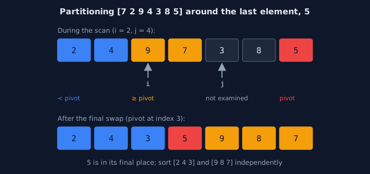
The partition invariant: a[lo:i] < pivot ≤ a[i:j], and a[j:hi-1] is not examined yet.
Lomuto Partition
// lomuto partitions a[lo:hi] around the pivot a[hi-1] and returns its final
// index p. Afterwards: a[lo:p] < pivot <= a[p+1:hi].
func lomuto(a []int, lo, hi int) int {
	pivot := a[hi-1]
	i := lo // a[lo:i] holds the elements smaller than the pivot
	for j := lo; j < hi-1; j++ {
		comparisons++
		if a[j] < pivot {
			a[i], a[j] = a[j], a[i]
			i++
		}
	}
	a[i], a[hi-1] = a[hi-1], a[i] // put the pivot between the two regions
	return i
}
Choosing the Pivot
If the pivot is always the smallest or largest element, one side is empty, recursion depth reaches n, and the cost is O(n²). A fixed choice such as "the last element" triggers this on input that is already sorted, which is common in practice. Swapping a random element into the pivot position makes the expected cost O(n log n) for every input. Recursing into the smaller side and looping on the larger one keeps the stack depth at O(log n).
| n = 4,000 (comparisons) | random input | sorted input | only 3 distinct values |
|---|---|---|---|
| last-element pivot | 53,703 | 7,998,000 | 2,670,615 |
| random pivot | 55,803 | 54,002 | 2,676,003 |
| random pivot, 3-way partition | 56,597 | 54,594 | 8,002 |
Many Duplicates: Three-Way Partitioning
The table shows a second weakness: with only three distinct values, even a random pivot is quadratic, because Lomuto puts every element equal to the pivot on the same side. The three-way partition (Dijkstra's Dutch national flag, seen in Arrays & Slices) splits the slice into less-than, equal-to, and greater-than regions. The equal region is finished in a single pass.
Quickselect
To find the k-th smallest element, such as the median or the 99th percentile, you do not need to sort. Partition once, then continue into only the side that contains index k. The expected work is n + n/2 + n/4 + … = O(n). The demo finds the median of a million values this way. container/heap's top-k pattern is O(n log k) but works on streams; quickselect needs all the data in memory.
Linear-Time Sorts
When keys are small integers, or split into small digits, you can use the key as an array index instead of comparing. Demo with a stability check against slices.SortStableFunc and timings: 35_linear_time_sorts.go.
Counting Sort
Count how many records have each key, turn the counts into starting positions with prefix sums (from Arrays & Slices), then place each record at its key's next free position. Walking the input in order keeps equal keys in order, so counting sort is stable. The cost is O(n + k) for keys in [0, k).
func countingSort(in []Student, k int) []Student {
	count := make([]int, k)
	for _, s := range in {
		count[s.grade]++
	}
	start := make([]int, k)
	for g := 1; g < k; g++ {
		start[g] = start[g-1] + count[g-1]
	}
	out := make([]Student, len(in))
	for _, s := range in {
		out[start[s.grade]] = s
		start[s.grade]++
	}
	return out
}
Radix Sort
Radix sort handles large keys by running a stable counting sort once per digit, from the least significant to the most significant. After pass d, the values are sorted by their lowest d digits. Stability preserves that order whenever later digits are equal. With 32-bit keys and 8-bit digits, that is four passes of O(n + 256). In the demo, radix sort is roughly eight to ten times faster than slices.Sort on random uint32 values. The costs are an O(n) buffer and a restriction to fixed-width integer (or string) keys.
Sorting in Go
In production code you write the ordering, not the sort. Demo with multi-key sorting, stable sorting, and searching by a custom key: 36_sorting_in_go.go.
slices.Sort and pdqsort
slices.Sort uses pdqsort (pattern-defeating quicksort). It combines ideas from this lesson: quicksort with careful pivot selection, insertion sort for short ranges, detection of already-sorted patterns, and a fallback to heapsort that guarantees O(n log n). It is not stable; use slices.SortStableFunc when you need stability.
Comparators and Multi-Key Orders
A comparison function returns a negative number, zero, or a positive number. cmp.Compare handles one key, and cmp.Or returns the first non-zero result, which gives multi-key ordering in a few lines:
// department ascending, then salary descending, then name
slices.SortFunc(staff, func(a, b Employee) int {
	return cmp.Or(
		cmp.Compare(a.Dept, b.Dept),
		cmp.Compare(b.Salary, a.Salary), // b before a: descending
		cmp.Compare(a.Name, b.Name),
	)
})
To search a slice sorted with a custom order, use slices.BinarySearchFunc with the same ordering. To rank records without moving them, sort a slice of indices and read the data through it.
Common Pitfalls
Sorting bugs rarely crash. They produce output that looks almost right.
Subtraction Comparators
return a - b overflows for large values, and the sort silently returns an unsorted slice. The demo shows this with math.MaxInt. Always use cmp.Compare, which also orders floating-point NaN values consistently.
Inconsistent Orderings
A comparator must define a consistent total order: if a < b and b < c, then a < c. A comparator with randomness, a time-dependent key, or a case-insensitive comparison mixed with a case-sensitive one breaks this, and the result is unspecified.
Assuming Stability
slices.Sort, slices.SortFunc, and sort.Slice are not stable. Code that sorts by one key and then by another only works with the stable variants.
Practice Lab
Before each exercise, decide which properties you need: stability, memory limit, worst-case guarantee, or key type.
Run the Demos
- In 32_elementary_sorts.go, change
a[j].rank > x.rankto>=ininsertionSortCards. The output is still sorted by rank. What changed? - In 33_merge_sort.go, replace
inv += len(l) - iwithinv++. The oracle catches it: explain which inversions are now missed. - In 34_quicksort.go, add
i++in thea[i] > pivotcase ofquickSort3Way. Why mustistay where it is after swapping withgt? - In 35_linear_time_sorts.go, run the radix passes from the most significant byte down (
shiftfrom 24 to 0). Why does it fail?
Exercises
- Merge intervals. Sort intervals by start, then merge overlapping ones in a single pass.
- Sort a linked list. Sort the
List[T]from Linked Lists in O(n log n) with merge sort. Use slow and fast pointers to find the middle. - Kth largest. Solve it three ways (sort, a heap of size k, quickselect) and time each for n = 10⁶ and k = 10 and k = n/2.
- Sort strings by length, then alphabetically. Once with a two-key comparator, once with two stable sorts. Which order must the two stable sorts run in?
Next: Graph Traversal.