Collections

This lesson covers the four containers you will use daily — arrays, tuples, dictionaries, and sets — then compares them side by side so the choice between them becomes obvious. It ends with the two pitfalls behind most collection bugs in Julia: aliasing through assignment, and untyped containers that quietly destroy performance.

Arrays

An array is an ordered, mutable container whose element type is fixed at construction. A one-dimensional array is a Vector; a two-dimensional one is a Matrix. Both are Array with a different number of dimensions, and everything you can do with a vector works for a matrix and for higher dimensions.

Constructing Arrays

The bracket syntax covers most cases, with the element type inferred from the values. When you need a specific type, or an empty container, state it — the default of an empty [] is Vector{Any}, which is almost never what you want.

# Element type is inferred from the values
v = [1, 2, 3]                 # Vector{Int64}
typeof(v)                     # Vector{Int64}

# Mixed types promote to a common type
[1, 2.5]                      # Vector{Float64} — [1.0, 2.5]
[1, "two"]                    # Vector{Any}    ⚠ the element type is lost

# Explicit element types
Int8[1, 2, 3]                 # Vector{Int8}
Float64[1, 2, 3]              # Vector{Float64}
String["a", "b"]              # Vector{String}

# Empty containers — always annotate
Int[]                         # Vector{Int64}, usable
[]                            # Vector{Any}  ⚠ avoid

# Sized and filled
zeros(3)                      # [0.0, 0.0, 0.0]
zeros(Int, 3)                 # [0, 0, 0]
ones(2, 3)                    # 2×3 matrix of 1.0
fill(7, 4)                    # [7, 7, 7, 7]

# Ranges become vectors on request
collect(1:5)                  # [1, 2, 3, 4, 5]
collect(1:2:9)                # [1, 3, 5, 7, 9]

Indexing, Slicing, and Views

Indexing uses square brackets with 1-based positions. Slicing returns a copy, while view returns a window that shares memory with the original — and the whole point of views is that they allocate nothing. Knowing which one you hold decides whether a mutation is visible to the caller.

v = [10, 20, 30, 40, 50]

v[1]              # 10      — first element
v[end]            # 50      — last element, whatever the length
v[end-1]          # 40
v[2:4]            # [20, 30, 40] — a COPY

# A slice is independent of the original
s = v[2:4]
s[1] = 99
v[3]              # 30 — unchanged, because s was a copy

# A view shares memory with the original
w = view(v, 2:4)      # w[1] is v[2], w[2] is v[3], w[3] is v[4]
w[1] = 99
v[2]              # 99 — changed: the view maps positions onto the same array
v[3]              # 30 — untouched, because w[1] is v[2], not v[3]

# Selection forms: ranges, masks, and index vectors
u = [10, 20, 30, 40, 50]
u[2:2:end]        # [20, 40] — indices 2 and 4
u[u .> 30]        # [40, 50] — a boolean mask
u[[1, 3]]         # [10, 30] — an index vector

u[6]              # ERROR: BoundsError — never returns garbage

# Dotted assignment writes into the selected positions
u[1:2] .= 0
u                 # [0, 0, 30, 40, 50]

Growing and Shrinking

push! and its relatives mutate in place, so the same name sees the new length. Growth is amortised — appending is fast on average — but a growth may relocate the array in memory, which is why a view taken earlier can be invalidated by a later push!.

v = Int[]

push!(v, 1)           # [1]
push!(v, 2, 3)        # [1, 2, 3] — several at once
append!(v, [4, 5])    # [1, 2, 3, 4, 5]
prepend!(v, [0])      # [0, 1, 2, 3, 4, 5]
insert!(v, 3, 99)     # [0, 1, 99, 2, 3, 4, 5]

pop!(v)               # returns 5; v is [0, 1, 99, 2, 3, 4]
popfirst!(v)          # returns 0; v is [1, 99, 2, 3, 4]
deleteat!(v, 2)       # [1, 2, 3, 4]

# Size queries and management
length(v)             # 4
size(v)               # (4,)
isempty(v)            # false
empty!(v)             # clears in place
v                     # Int64[] — the element type is preserved

# Pre-allocate when you know roughly how large the array will be
sizehint!(Int[], 1_000)
resize!([1, 2, 3], 5) # length 5 — but the NEW elements are uninitialised ⚠

# Never read the elements that resize! added:
v2 = [1, 2, 3]
resize!(v2, 5)        # v2[4] and v2[5] may hold arbitrary garbage
v2[4]                 # some Int, possibly not 0 — do not rely on it
v2[4:5] .= 0          # zero only the positions you added
fill!(v2, 0)          # or zero the whole array, deliberately

Multidimensional Arrays

A matrix literal separates columns with spaces and rows with semicolons. Because the data is stored column-major, the first index varies fastest, and that single fact explains linear indexing, eachcol versus eachrow, and the loop-order advice from the Loops lesson.

A = [1 2; 3 4]          # 2×2 matrix
A = [1 2
     3 4]               # the same matrix, written over two lines

size(A)                 # (2, 2)
length(A)               # 4  — total elements
axes(A)                 # (Base.OneTo(2), Base.OneTo(2))

A[1, 1]                 # 1 — row 1, column 1
A[2, 1]                 # 3 — row 2, column 1
A[1, :]                 # [1, 2] — the whole first row
A[:, 1]                 # [1, 3] — the whole first column (contiguous!)

# Linear indexing follows column-major order
A[1]                    # 1
A[2]                    # 3  — the second element of column 1
A[3]                    # 2  — the first element of column 2

# Matrix arithmetic versus element-wise work
[1 2; 3 4] * [1, 2]     # [5, 11] — matrix × vector
A .+ 1                  # [2 3; 4 5] — element-wise
A'                      # [1 3; 2 4] — adjoint (conjugate transpose)
transpose(A)            # [1 3; 2 4] — transpose without conjugation

# Reductions along an axis keep the dimension: the result is a matrix
sum(A, dims = 1)        # [4 6] — a 1×2 matrix: column sums (size (1, 2))
sum(A, dims = 2)        # a 2×1 matrix — row sums, printed as [3; 7;;]
reshape([3, 7], 2, 1)   # the explicit way to write that 2×1 shape
sum(A)                  # 10 — a scalar: the total
dropdims(sum(A, dims = 1), dims = 1)   # [4, 6] — a vector, if you want one

# Iterating and reshaping
reshape(1:6, 2, 3)      # 2×3 matrix filled column-major
vec([1 2; 3 4])         # [1, 3, 2, 4] — flatten in memory order
collect(eachcol(A))     # [[1, 3], [2, 4]] — columns
collect(eachrow(A))     # [[1, 2], [3, 4]] — rows

Tuples

A tuple is an ordered, immutable sequence written with parentheses. Because it cannot change size or contents after construction, the compiler knows everything about it: a tuple is stored inline, its length is part of its type, and its fields are addressed at compile time. This makes tuples the natural way to return several values from a function.

Immutable, Ordered, and Fast

A tuple may mix types without losing performance — (1, "two") has type Tuple{Int64, String}, which is fully concrete. This is the opposite of an array, where mixing types forces Vector{Any}.

t = (1, 2, 3)
typeof(t)             # Tuple{Int64, Int64, Int64}
length(t)             # 3

# A one-element tuple needs a trailing comma
one = (42,)           # Tuple{Int64}
not_a_tuple = (42)    # just the number 42

# Mixed types stay concrete — no boxing
m = (1, "two", 3.0)
typeof(m)             # Tuple{Int64, String, Float64}

# Indexing starts at 1, exactly as for arrays
t[1]                  # 1
t[end]                # 3

# Immutability is enforced
t[1] = 99             # ERROR: MethodError: no method matching setindex!

# Tuples are comparable and hashable
(1, 2) == (1, 2)      # true
(1, 2) < (1, 3)       # true — lexicographic
Dict((1, 2) => "a")[(1, 2)]   # "a" — usable as a dictionary key

# Build one from a collection when you need fixed arity
Tuple([1, 2, 3])      # (1, 2, 3)

Destructuring and Splatting

Destructuring assigns the parts of a tuple, and of any iterable, to separate names in one statement. It is how multiple return values are received, how two variables are swapped, and how the head and tail of a sequence are separated.

# Positional destructuring
t = (1, "two", 3.0)
a, b, c = t
a                     # 1
b                     # "two"

# The last name may collect the remainder
first_item, rest... = (1, 2, 3, 4)
first_item            # 1
rest                  # (2, 3, 4) — a tuple

# Swapping without a temporary
x, y = 1, 2
x, y = y, x
x, y                  # (2, 1)

# Nested destructuring
(a, (b, c)) = (1, (2, 3))
b, c                  # (2, 3)

# Receiving several return values from a function
function minmax(v)
    (minimum(v), maximum(v))
end
lo, hi = minmax([3, 1, 4, 1, 5])
lo, hi                # (1, 5)

# Looping over pairs of a dictionary destructures naturally
for (k, v) in Dict(:a => 1, :b => 2)
    println("$k = $v")
end

# Underscore marks a value you do not need
_, second = (10, 20)
second                # 20

Named Tuples

A named tuple gives each field a name while keeping tuple semantics: immutable, inline, and ordered. It is the lightweight alternative to defining a struct — ideal for a row of data, a configuration record, or an option bundle that never needs methods of its own.

nt = (name = "Ada", age = 36)
typeof(nt)            # @NamedTuple{name::String, age::Int64}

nt.name               # "Ada" — field access by name
nt.age                # 36
nt[1]                 # "Ada" — positional access still works
nt[:name]             # "Ada" — and by symbol

keys(nt)              # (:name, :age)
values(nt)            # ("Ada", 36)
length(nt)            # 2
nt == (name = "Ada", age = 36)    # true — structural equality

# Building one from existing values, and extending one
base = (x = 1, y = 2)
extended = (; base..., z = 3)     # (x = 1, y = 2, z = 3)
merge(base, (y = 20,))            # (x = 1, y = 20)

# A missing field is an error, not nothing
nt.height             # ERROR: type @NamedTuple{...} has no field height
haskey(nt, :height)   # false — test before reaching

# Named tuples make function returns self-documenting
function measure(v)
    (min = minimum(v), max = maximum(v), n = length(v))
end
m = measure([3, 1, 4])
m.min                 # 1
m.n                   # 3

Dictionaries

A dictionary maps keys to values with expected constant-time lookup. Keys must be hashable — strings, symbols, numbers, tuples, and immutable structs all qualify. The iteration order is not the insertion order. It is determined by the hash table and may change between runs or versions, so never rely on it.

Creating and Accessing

The literal form uses key => value pairs. Reading a missing key raises KeyError; every safe way to read is a named function, which is a deliberate design choice: the dangerous operation is the short one, so passing a bad key is loud rather than silent.

d = Dict("a" => 1, "b" => 2)
typeof(d)             # Dict{String, Int64}

# Explicitly typed, empty
empty_typed = Dict{String, Int}()

d["a"]                # 1
d["zzz"]              # ERROR: KeyError: key "zzz" not found

# Safe reads
haskey(d, "a")        # true
get(d, "a", 0)        # 1
get(d, "zzz", 0)      # 0 — the default is returned, and nothing is inserted

# ⚠ There is no two-argument get for a dictionary — this is an error, not
#   a way to ask "is it there?":
get(d, "zzz")         # ERROR: MethodError
get(d, "zzz", nothing)   # ✅ the explicit way to get nothing back

# Writing and updating
d["c"] = 3            # insert or overwrite
push!(d, "d" => 4)    # the same thing, as a Pair
merge(d, Dict("e" => 5))          # a NEW dict with the keys combined
merge!(d, Dict("e" => 5))         # merges into d

# get! inserts on demand — the memoisation pattern in one call
counts = Dict{String, Int}()
get!(counts, "apple", 0)          # 0, and the key now exists
counts["apple"] += 1
counts["apple"]                   # 1

# Removing
delete!(d, "a")                   # d is now without "a"
pop!(d, "b", "missing")           # returns the value, or the fallback

Iterating a Dictionary

Iterating a dictionary yields Pairs, which destructure into keys and values. For keys or values alone, keys and values return lazy views rather than copies.

d = Dict("a" => 1, "b" => 2, "c" => 3)

# Pairs, destructured at the loop head
for (k, v) in d
    println("$k → $v")            # order is hash order, not insertion order
end

# Keys and values as views
collect(keys(d))                  # ["a", "b", "c"] in hash order
collect(values(d))                # the matching values
sort(collect(keys(d)))            # ["a", "b", "c"] — impose your own order

# Iterate in a defined order by sorting first
for k in sort(collect(keys(d)))
    println("$k = $(d[k])")
end

# Transformations keep dictionaries dictionaries
Dict(k => v * 10 for (k, v) in d)          # scaled values
filter(p -> p.second > 1, d)               # keeps "b" and "c"
map(uppercase, collect(keys(d)))           # ["A", "B", "C"]

# Size and emptiness
length(d)                         # 3
isempty(d)                        # false
empty!(d)                         # clears in place, type preserved

Sets

A set is an unordered collection of unique elements with expected constant-time membership testing. Use it when the question is "is this here?" or "what is unique?" — the two operations it exists for, and the two that arrays do slowly.

Set Operations

Julia ships the full algebra: union, intersection, difference, symmetric difference, and subset tests. All of them return new sets; the mutating variants exist separately with the usual ! suffix.

s = Set([1, 2, 3])            # Set{Int64} — duplicates are dropped
push!(s, 4)                   # Set([1, 2, 3, 4])
push!(s, 4)                   # still four elements — adding a duplicate is a no-op

length(s)                     # 4
2 in s                        # true  — membership is the point
10 in s                       # false

# The algebra
union(Set([1, 2]), Set([2, 3]))          # Set([1, 2, 3])
intersect(Set([1, 2, 3]), Set([2, 3, 4]))# Set([2, 3])
setdiff(Set([1, 2, 3]), Set([2]))        # Set([1, 3])
symdiff(Set([1, 2]), Set([2, 3]))        # Set([1, 3]) — in one but not both
issubset(Set([1, 2]), Set([1, 2, 3]))    # true
isdisjoint(Set([1]), Set([2]))           # true

# Mutating variants modify the first argument
union!(Set([1, 2]), [3])                 # Set([1, 2, 3])
setdiff!(Set([1, 2, 3]), [2])            # Set([1, 3])

# Elements must be hashable. Hashing follows content, not identity, so equal
# immutable values — and equal arrays — collapse into one member:
Set([(1, 2), (1, 2)])                    # Set with 1 element — tuples compare by value
Set([[1, 2], [1, 2]])                    # Set with 1 element too ⚠ arrays also hash by content
Set([[1, 2], [3, 4]])                    # Set with 2 elements — different contents

d = Dict([1, 2] => "a")
d[[1, 2]]                 # "a" — found by content hash

k = first(keys(d))        # the array stored as the key
push!(k, 3)               # k is now [1, 2, 3] — its hash just changed
k                         # [1, 2, 3]
d[[1, 2]]                 # ERROR: KeyError — the entry is now unreachable
d[[1, 2, 3]]              # ERROR too — the table still holds the old hash

Membership, Deduplication, and Order

Sets do not preserve insertion order, so converting a vector to a set and back is a lossy round trip for anything order-sensitive. When order matters but duplicates do not, unique keeps the first occurrence in place.

v = [3, 1, 3, 2, 1]

unique(v)                     # [3, 1, 2] — order preserved, first wins
collect(Set(v))               # some order, guaranteed only to be unique

# Deduplicate while keeping order: the idiom is a set of seen values
function unique_ordered(v)
    seen = Set{eltype(v)}()
    out = eltype(v)[]
    for x in v
        if !(x in seen)
            push!(seen, x)
            push!(out, x)
        end
    end
    out
end
unique_ordered([3, 1, 3, 2, 1])           # [3, 1, 2]

# Membership is O(1) for a Set and O(n) for a Vector — this is the whole
# reason to build one:
large = Set(1:1_000_000)
500_000 in large                           # true, found by hashing
500_000 in collect(large)                  # also true, but this scans the array

# Set operations answer set-shaped questions concisely
words = Set(["apple", "fig"])
"fig" in words                             # true
length(intersect(words, Set(["fig", "plum"])))   # 1 — how many are shared

Choosing a Container

The four containers differ in four properties: whether they are ordered, whether they change, whether duplicates are allowed, and what the element type may be. Deciding which property matters most usually decides the container.

Comparison Table

Two rules of thumb follow from the table. If you need to look things up by a value that is not a small integer, build a Dict or a Set rather than searching an array. If a group of values always travels together and never changes, a Tuple or NamedTuple is cheaper than a struct and clearer than parallel arrays.

Converting Between Containers

Conversion functions are constructors and collectors: collect builds an array, and the container name itself builds the other kinds. Each conversion is a real copy — nothing is shared with the original.

v = [3, 1, 3, 2]

collect(1:4)                  # [1, 2, 3, 4] — range to vector
Set(v)                        # Set([3, 1, 2]) — duplicates dropped
Tuple(v)                      # (3, 1, 3, 2) — fixed size, immutable
Dict(1:3 .=> ["a", "b", "c"])  # Dict(1 => "a", 2 => "b", 3 => "c")
sort(v)                       # [1, 2, 3, 3] — a sorted COPY
collect(keys(Dict(:a => 1)))  # [:a] — dictionary keys to a vector

# A vector of pairs becomes a dictionary directly
Dict(["a" => 1, "b" => 2])     # Dict{String, Int64}
Dict(:a => 1, :b => 2)         # the same, with symbols

# A matrix and a vector are different shapes, not different data
vec([1 2; 3 4])               # [1, 3, 2, 4] — flatten, column-major
reshape([1, 2, 3, 4], 2, 2)   # [1 3; 2 4] — the same memory, reinterpreted

Memory and Performance Notes

Three facts explain most collection performance in Julia, and all three follow from the type system rather than from tuning.

• Element type decides layout. Vector{Int} stores its values contiguously with no per-element overhead; Vector{Any} stores pointers to boxed objects, so every access is an indirect one.
• Fixed-size beats growable when the size is known. A tuple never reallocates, and a Dict or Set hashes each key — cheap, but more work per element than an index.
• Column-major order drives iteration. The first index varies fastest, as the Loops lesson demonstrated: walking that index in the inner loop can be about twice as fast on large matrices.

Common Pitfalls

Copy versus Alias

Assignment never copies. b = a binds a second name to the same array, so a mutation through either name is visible through both. copy makes an independent array. This is the single most common surprise for programmers arriving from a value-semantics language.

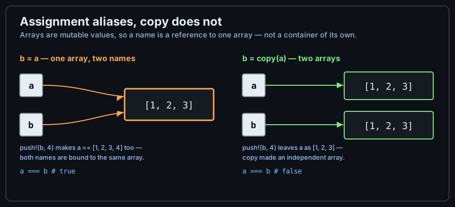
Two names, one array on the left; two independent arrays on the right. a === b tells you which situation you are in.

a = [1, 2, 3]
b = a                 # alias: the same array
b[1] = 99
a                     # [99, 2, 3] — a changed too
a === b               # true

c = copy(a)           # independent
c[1] = 0
a                     # [99, 2, 3] — unchanged
a === c               # false

# A function that mutates its argument changes the caller's array:
function double!(v)
    v .*= 2
end
double!(a)
a                     # [198, 4, 6]

# copy is SHALLOW: a vector of vectors shares the inner ones
inner = [1, 2]
outer = [inner, inner]
shallow = copy(outer)
shallow[1][1] = 99
inner                 # [99, 2] — the inner array is shared
deepcopy(outer)[1][1] = 0     # deepcopy breaks every level
inner                 # [99, 2] — unaffected by deepcopy's result

Vector{Any} from a Mixed Literal

One value of an unexpected type is enough to strip the element type from a whole array. It usually enters through a literal, a comprehension with inconsistent branches, or an empty [] that was filled later. The fix is local and cheap: convert at the boundary where untyped data arrives.

# ❌ One string turns the whole array untyped
data = [1, 2, "three"]        # Vector{Any}
eltype(data)                  # Any

# ❌ A comprehension whose branches disagree loses the type too
label(x) = x > 0 ? x : "non-positive"
[label(i) for i in [1, -2, 3]]     # Vector{Any}

# ❌ An untyped empty vector
acc = []
push!(acc, 1.5)
eltype(acc)                   # Any — every push boxes

# ✅ Keep branches the same type, or convert explicitly at the boundary
parsed = [parse(Float64, s) for s in ["1.5", "2.5"]]   # Vector{Float64}
eltype(parsed)                # Float64

# ✅ Annotate empty containers
acc2 = Float64[]
push!(acc2, 1.5)
eltype(acc2)                  # Float64

# ✅ When untyped data is unavoidable, convert once — then it is typed
mixed = Any[1, 2, 3]
numbers = Float64[Float64(x) for x in mixed]           # Vector{Float64}

KeyError and Missing Keys

Square brackets on a dictionary are a promise that the key exists, and breaking that promise raises KeyError. The safe alternatives cover the three things you actually mean: a fallback value, an on-demand insert, or an explicit test.

d = Dict(:a => 1)

d[:b]                     # ERROR: KeyError: key :b not found

# Three ways to say what you meant
get(d, :b, 0)             # 0 — a fallback, leaving d unchanged
get!(d, :b, 0)            # 0 — and now d[:b] exists
haskey(d, :b)             # true — after the get! above

# Counting with get! avoids both a KeyError and a branch
counts = Dict{Char, Int}()
for c in "abracadabra"
    counts[c] = get(counts, c, 0) + 1
end
counts['a']               # 5

# The same loop with a default-returning dictionary is shorter
counts2 = Dict{Char, Int}()
for c in "abracadabra"
    get!(counts2, c, 0)
    counts2[c] += 1
end
counts2['b']              # 2

# Sorting the keys first gives a deterministic report
for c in sort(collect(keys(counts)))
    println("$c = $(counts[c])")
end

You now have the full set of everyday containers and the rules that pick between them. The next phase moves from values to behaviour: Strings & Text handles text properly, then types and modules let you define your own abstractions.