Loops & Iteration

This lesson covers the two loop forms and the protocol beneath them, the helpers that remove manual counters, the ways to leave or skip an iteration, and the comprehension and generator forms that replace most short loops entirely. It ends with the performance rules that matter most in Julia: type stability, memory order, and why a loop at global scope can run hundreds of times slower than the identical loop inside a function.

for Loops

The for loop binds a name to each element of an iterable in turn. There is no initialisation clause, no condition, and no increment step — those are properties of the range you choose, not of the loop. The body is terminated by end.

# Iterating a range — the closest thing to a classical counting loop
for i in 1:5
    println(i)           # prints 1 2 3 4 5
end

# Iterating a collection: you get the element, not the index
for fruit in ["apple", "pear", "plum"]
    println(uppercase(fruit))
end

# `in` and `=` are interchangeable here, and ∈ is the mathematical spelling
for i = 1:3;  print(i); end
for i ∈ 1:3;  print(i); end

Ranges and Steps

A range is a value in its own right, not a loop construct. Once you know the three literals — a:b, a:s:b, and the range() function — you can build any counting sequence without touching the loop.

collect(1:5)              # [1, 2, 3, 4, 5]
collect(1:2:9)            # [1, 3, 5, 7, 9]
collect(5:-1:1)           # [5, 4, 3, 2, 1]

length(1:5)               # 5 — O(1), the range is not materialised
sum(1:5)                  # 15 — ranges compose with any reducer

# Floating-point ranges never accumulate rounding error:
collect(range(0, 1, length = 5))     # [0.0, 0.25, 0.5, 0.75, 1.0]

# ⚠ A missing sign produces an EMPTY range, not an error:
collect(5:1)              # Int64[] — the loop body never runs
collect(5:-1:1)           # [5, 4, 3, 2, 1]

That last warning is the most common loop bug in Julia: 5:1 is a legitimate but empty range, so a descending loop that forgot the -1 step silently does nothing at all.

The Iteration Protocol

What makes for x in thing work is a small protocol, not a language feature: the loop calls iterate(thing) to start and keeps calling iterate(thing, state) until it returns nothing. Anything that implements those two methods is iterable — including your own types.

# Built-in iterables, all driven by the same protocol
for c in "abc";      print(c); end        # abc   — a String iterates characters
for k in Dict(:a => 1); print(k); end     # :a=>1 — a Dict iterates Pairs
for (k, v) in Dict(:a => 1); print("$k=$v"); end   # a=1 — each Pair destructures

# A custom iterable needs only these two methods:
struct Countdown
    from::Int
end
# Stop at 1, otherwise the sequence 3,2,1 would continue with a final 0.
Base.iterate(c::Countdown, i = c.from) = i < 1 ? nothing : (i, i - 1)

for n in Countdown(3); print(n); end      # 321

# collect also needs a length, because it must allocate the result first:
Base.length(c::Countdown) = c.from
collect(Countdown(3))                     # [3, 2, 1]

Note the asymmetry: a for loop needs only iterate, because it walks the sequence one element at a time. Functions that must allocate — collect, length, sizehint! — also need length or an IteratorSize declaration.

Because iteration is a protocol rather than a fixed list of acceptable types, the same loop body works on arrays, ranges, dictionaries, generators, file lines, and network streams. That is why Julia code contains far fewer loop variants than you might expect.

eachindex and CartesianIndices

When you genuinely need indices, do not compute them by hand. eachindex returns the indices that are valid for the object you actually have, which matters for arrays whose first index is not 1. For multidimensional work, CartesianIndices gives you tuples of indices and keeps the memory order correct.

v = [10, 20, 30]

# ✅ Ask the array what its indices are
for i in eachindex(v)
    v[i] *= 2
end
v                          # [20, 40, 60]

# ❌ Hard-coded indices break the moment someone passes an OffsetArray
for i in 1:length(v)
    v[i] *= 2
end

# Multidimensional: CartesianIndices yields index tuples in memory order
B = [1 2; 3 4]
for I in CartesianIndices(B)
    B[I] += 1              # I is a CartesianIndex, usable directly as B[I]
end
B                          # [2 3; 4 5]

# A range of indices is also a CartesianIndex shortcut:
for I in CartesianIndices((2, 2)); B[I] = 0; end

enumerate and zip

Two helpers remove the most common reasons for falling back to manual indexing. enumerate pairs each element with its position; zip walks several collections in lockstep. Both are lazy — they produce tuples on demand rather than building intermediate arrays.

# enumerate: index and element together, always starting at 1
for (i, fruit) in enumerate(["apple", "pear", "plum"])
    println("$i: $fruit")        # 1: apple, 2: pear, 3: plum
end

# enumerate has no `start` keyword — for a 0-based index, zip a range instead
for (i, x) in zip(0:2, "abc")
    println("$i → $x")           # 0 → a, 1 → b, 2 → c
end

# Or subtract one from enumerate's index:
for (i0, x) in enumerate("abc")
    println("$(i0 - 1) → $x")    # 0 → a, 1 → b, 2 → c
end

# zip: same position across several collections, stopping at the shortest
names = ["a", "b", "c"]
scores = [10, 20, 30]
for (n, s) in zip(names, scores)
    println("$n scored $s")
end

# Three or more collections zip just as easily
for (i, n, s) in zip(1:3, names, scores)
    println("$i $n $s")
end

# zip is lazy, so it can pair a large range with a short array safely
collect(zip(1:100, ["x", "y"]))    # [(1, "x"), (2, "y")] — length 2

Because zip stops at the shortest input, it cannot produce an out-of-bounds access — but it can hide a length mismatch. When the lengths must agree, check them explicitly with @assert length(a) == length(b) before the loop.

while Loops

A while loop repeats as long as its condition is true. It is the right form when the number of iterations is not known in advance — reading until end of input, iterating until convergence, walking a linked structure. The condition must be a real Bool, exactly as in if.

while and the Loop Variable

The loop variable is not part of the syntax; you maintain it yourself. That extra responsibility is the source of the classic infinite loop, so always ask what makes the condition false.

n = 5
while n > 0
    println(n)
    n -= 1               # ← without this the loop never ends
end

# A convergence loop: iterate until the change is negligible
x = 1.0
while abs(x - cos(x)) > 1e-12
    x = cos(x)
end
x                        # 0.7390851332151607 — the Dottie number

# Iterating with an explicit state that is not a counter
queue = [1, 2, 3]
while !isempty(queue)
    item = popfirst!(queue)
    item < 3 && push!(queue, item + 10)   # 1 → 11, 2 → 12
end

Emulating do-while

Julia has no do…while, and it does not need one: a while true loop with a break at the bottom gives exactly the body-first semantics, and it works for conditions that need variables computed inside the body.

# Run the body once, then decide.
attempts = 0
while true
    attempts += 1
    ok = attempts ≥ 3          # imagine a real operation here
    ok && break                # ← the do-while condition, at the bottom
    println("retry $attempts")
end
attempts                       # 3

# `do` is a different keyword: it attaches a function to a call.
open("data.txt", "w") do io
    println(io, "hello")
end

Deliberate Infinite Loops

Some loops are meant to run until an external event stops them. Write those as while true and make the exit paths obvious; a bare while true with the exit buried inside helper calls is a maintenance hazard.

# A server-style loop: exit only on an explicit signal.
function pump(iterations)
    count = 0
    while true
        count += 1
        count ≥ iterations && return count   # one, clearly visible exit
    end
end
pump(4)          # 4

# For a finite but unknown count, prefer a bounded loop:
for _ in 1:10_000
    # give up after 10 000 attempts rather than spin forever
end

Controlling a Loop

Two keywords inside a loop body change the flow: break leaves the innermost loop immediately, and continue skips the rest of the current iteration. Both are ordinary to reach for, but Julia deliberately omits labelled breaks — the idiomatic replacement is a function.

break and continue

break is how a loop answers yes and stops; continue is how it discards an element and moves on. Used together they let a flat loop body express filtering and early exit without extra indentation.

# break: stop as soon as the answer is known
target = 7
for x in 1:100
    if x^2 ≥ target
        println("first square ≥ $target is $(x^2)")   # 9
        break
    end
end

# continue: skip elements that do not matter, without nesting the rest
total = 0
for x in 1:20
    x % 2 == 0 && continue            # ignore evens
    x > 15 && break                    # stop past 15
    total += x
end
total                                  # 1+3+5+7+9+11+13+15 = 64

# `x % 2 == 0 && continue` is the compact guard form; the block form is:
for x in 1:20
    if x % 2 == 0
        continue
    end
end

Nested Loops and the Missing Label

Julia has no labelled break, so break inside a nested loop exits only the inner loop. There are three clean ways out: put the search in a function and return, use a flag, or restructure with any/all.

grid = [1 2 3; 4 5 6; 7 8 9]

# ❌ break only leaves the inner loop — the outer loop keeps going
for i in 1:3
    for j in 1:3
        grid[i, j] == 5 && break          # stops j, not i
    end
end

# ✅ Wrap the search in a function: return exits both loops at once
function find_value(g, target)
    for i in axes(g, 1), j in axes(g, 2)
        g[i, j] == target && return (i, j)
    end
    return nothing
end
find_value(grid, 5)          # (2, 2)

# ✅ Or let a predicate do the work — any() stops at the first hit
any(==(5), grid)             # true
findfirst(==(5), grid)       # CartesianIndex(2, 2)

The Value of a Loop

Unlike if, a loop evaluates to nothing. You cannot write x = for … end and expect a result. Loops exist for their side effects, so the accumulated value must be produced by a comprehension, a map/reduce call, or an accumulator you update yourself.

# A loop is worth nothing:
r = for i in 1:3; i^2; end
r                            # nothing

# Three idiomatic ways to produce a value instead:
squares = [i^2 for i in 1:3]          # [1, 4, 9]   — comprehension
squares2 = map(i -> i^2, 1:3)         # [1, 4, 9]   — map
total = sum(i^2 for i in 1:3)         # 14          — generator + reducer

# Or accumulate explicitly — the clearest form when the body is complex:
acc = 0
for i in 1:3
    acc += i^2
end
acc                          # 14

Comprehensions and Generators

Most short loops exist to build a collection from another collection. Julia has a dedicated form for exactly that task, and it is both shorter and faster than the loop: the comprehension. Its lazy twin, the generator, avoids allocating the result at all.

Array Comprehensions

A comprehension is written like a loop with the body in front, enclosed in square brackets. Conditions may be appended, and multiple for clauses nest in the order written.

# Body first, then the iteration
squares = [i^2 for i in 1:5]                  # [1, 4, 9, 16, 25]

# With a filter — the condition is not a branch, it is a filter
evens = [i for i in 1:10 if iseven(i)]        # [2, 4, 6, 8, 10]

# A transformation plus a filter
words = ["apple", "fig", "banana", "kiwi"]
long_upper = [uppercase(w) for w in words if length(w) > 4]
long_upper                                    # ["APPLE", "BANANA"]

# Nested clauses read left to right, the outer loop first
pairs = [(i, j) for i in 1:2 for j in 1:2]    # [(1,1), (1,2), (2,1), (2,2)]

# The result type follows the body
[Int(x) for x in [1.0, 2.5]]                  # throws InexactError for 2.5

# round(Int, x) converts explicitly — and rounds halves to the nearest EVEN
# number, so 2.5 becomes 2 while 3.5 becomes 4 (banker's rounding):
[round(Int, x) for x in [1.0, 2.5]]           # [1, 2]
[round(Int, x) for x in [1.0, 3.5]]           # [1, 4]

# Ask for the other convention when you need it:
[round(Int, x, RoundNearestTiesAway) for x in [2.5, 3.5]]    # [3, 4]

A comprehension always materialises its result. When the body is expensive and you only need the values one at a time, a generator is the better choice.

Generators (Lazy)

Drop the square brackets and you get a generator: the same expression, evaluated on demand. Generators are the argument of choice for sum, maximum, any, all, and mapreduce, because nothing is allocated for the intermediate sequence.

# No brackets: nothing is built, values arrive one by one
g = (i^2 for i in 1:5)
collect(g)                     # [1, 4, 9, 16, 25] — pulling forces evaluation

# The idiomatic consumer forms
sum(i^2 for i in 1:5)          # 55
maximum(i^2 for i in 1:5)      # 25
any(i > 4 for i in 1:5)        # true — stops at the first true
all(i > 0 for i in 1:5)        # true

# A generator over a huge range is safe: nothing is materialised
sum(i for i in 1:10^9)         # runs in constant memory

map, filter, and their friends

When you already have a named function, the higher-order forms read better than a comprehension. They also make the intent explicit — filter says "keep these", map says "transform each" — and compose with |>.

v = [1, 2, 3, 4, 5, 6]

map(x -> x^2, v)               # [1, 4, 9, 16, 25, 36]
filter(iseven, v)              # [2, 4, 6]
filter(!iseven, v)             # [1, 3, 5]

# Two-argument map walks two collections in parallel
map(+, [1, 2, 3], [10, 20, 30])     # [11, 22, 33]

# Reducers
sum(v)                         # 21
prod([1, 2, 3, 4])             # 24
maximum(v)                     # 6
count(iseven, v)               # 3

# mapreduce fuses the two: transform, then reduce, without a temporary array
mapreduce(x -> x^2, +, v)      # 91 = 1+4+9+16+25+36

# Piping composes left to right and reads like a sentence
v |> x -> filter(iseven, x) |> x -> map(x -> x * 10, x)   # [20, 40, 60]

Broadcasting Is an Implicit Loop

The dotted operators from the previous lesson are the fourth way to express "for each element": shorter than a comprehension, allocation-free thanks to fusion, and applicable to any function. Choose broadcasting when the operation is element-wise and shape-preserving, and a comprehension when you need to filter, nest, or change shape.

v = [1, 2, 3, 4, 5, 6]

# All four forms produce the same result — pick by intent
[i^2 for i in v]               # comprehension: explicit
map(x -> x^2, v)               # map: a named transformation
v .^ 2                         # broadcast: element-wise operator
broadcast(x -> x^2, v)         # broadcast: long form

# Broadcasting wins when the expression has several steps:
y = @. v^2 + 3v + 1            # one fused pass, no temporaries

Loop Performance

A loop in one language is not a loop in another. Julia compiles loops to machine code, so the difference between a fast loop and a slow one is rarely the algorithm — it is whether the compiler had enough type information, and whether the memory access pattern matched how the data is laid out.

Type Stability

A function is type-stable when the compiler can infer the type of every variable from the types of the arguments alone. When it cannot, values are boxed on the heap and every operation becomes a run-time dispatch. The classic cause is a variable that starts with no type information — most often an empty container written as [] instead of Float64[].

# ❌ `[]` is a Vector{Any}: every push boxes a Float64 and every read unboxes it
function any_accumulator(v)
    out = []
    for x in v
        push!(out, x / 2)
    end
    sum(out)
end

# ✅ A concrete element type: no boxing, one tight loop
function typed_accumulator(v)
    out = Float64[]
    for x in v
        push!(out, x / 2)
    end
    sum(out)
end

# Measured on a million elements, the first version is about 8× slower —
# same answer, different amount of work per element.

Not every inferred union is expensive, and it is worth knowing the difference. If a variable takes one of two or three concrete types, Julia applies union splitting: it compiles a specialised path per type and branches once. That is why the following loop, despite being technically unstable, runs at essentially full speed.

# Unstable in theory: `acc` is Union{Int64, Float64} — it starts as Int
# and is promoted on the first iteration.
function total_bad(v)
    acc = 0
    for x in v
        acc = acc + x / 2
    end
    acc
end

# Stable: initialise with the type it will keep.
function total_good(v)
    acc = 0.0
    for x in v
        acc += x / 2
    end
    acc
end

# Both run at the same speed (a two-type union is split at compile time),
# but only the second one is easy to reason about — and only the second
# survives if the body grows and the union becomes larger.

using Test
@inferred total_good([1, 2, 3])       # passes: inference produced one concrete type
# @inferred total_bad([1, 2, 3])      # fails: the return type is a Union

Use @code_warntype to see what the compiler inferred — unstable variables are highlighted — and @inferred in your tests to assert stability where it matters. The habit that pays off most is simply annotating empty containers: Float64[], Int[], or Vector{MyType}().

Memory Order

Julia arrays are stored in column-major order — the same convention as Fortran and R, and the opposite of C. The first index varies fastest in memory, so a loop that walks the first index in its innermost loop reads memory sequentially and lets the CPU prefetch. Swap the two loops and you stride through memory instead, which costs cache misses while producing identical results.

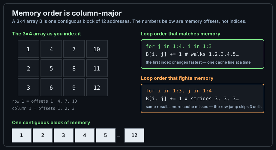
Addresses increase down each column, so the inner loop should advance the first index. The two loops below compute the same answer; only one of them walks memory in order.

B = rand(1000, 1000)

# ✅ Column-major friendly: i (the first index) varies fastest
function column_major(B)
    s = 0.0
    for j in axes(B, 2), i in axes(B, 1)
        s += B[i, j]
    end
    s
end

# ❌ Row-major thinking: striding across columns on every step
function row_major(B)
    s = 0.0
    for i in axes(B, 1), j in axes(B, 2)
        s += B[i, j]
    end
    s
end

# Both give the same sum. On a 1500×1500 array the column-major version
# measured about twice as fast — the difference is cache behaviour, not maths.

# When the loop body needs no indices at all, avoid them entirely:
sum(B)                                  # the built-in is already optimal

Global Scope Is the Real Trap

The largest and most surprising slowdown in Julia is not in the loop at all — it is where the data lives. A non-const global may be reassigned to a different type at any moment during a session, so the compiler is not allowed to assume its type. Every access becomes a dynamic lookup, and the loop stays slow whether it runs at top level or inside a function.

gv = collect(1:1_000_000)          # a non-const global (no `const`)

# ❌ At top level: ≈169 ms measured for this million-element loop.
s = 0
for x in gv
    global s += x                  # `for` is a soft scope: `global` is needed
end

# ❌ Even inside a function, reading a non-const global keeps it slow:
function slow()
    s = 0
    for x in gv                    # read from the enclosing global scope
        s += x
    end
    s
end
slow()                             # ≈69 ms — still a dynamic lookup per access

# ✅ Passing the value in as an argument makes the function specialised,
#    whether or not the caller's variable was const: ≈0.3 ms.
function fast(v)
    s = 0
    for x in v
        s += x
    end
    s
end
const GV = collect(1:1_000_000)
fast(GV)                           # same answer, compiled to machine code — ~500× faster

# ✅ The other idiomatic fix: wrap the work in a let block, which creates
#    an ordinary local variable bound to the global's value.
let v = GV
    total = 0
    for x in v
        total += x
    end
    total
end

@simd and Vectorisation

Modern CPUs execute several independent arithmetic operations per cycle. For a reduction whose operations are associative — summing floats is associative in exact arithmetic, though not in floating point — you can invite the compiler to reorder the loop with @simd. It is a hint about reordering, not a promise about accuracy, so use it when a small change in the last digits is acceptable.

function sum_simd(v)
    s = 0.0
    @simd for x in v               # allow the compiler to use vector instructions
        s += x
    end
    s
end

# The macro asserts that reordering is legal. It is not free:
#   * the result may differ in the last bits from a strictly ordered sum
#   * it does nothing if the loop body is not amenable to vectorisation

# For element-wise work, broadcasting already produces the tight loop:
y = @. 2 * v .+ 1                  # no loop written, no temporary allocated

Common Pitfalls

Off-by-One and the 1-Based Index

Julia indexes from 1. Index 0 is out of bounds, and there is no "valid but harmless" zero element — a C-style loop starting at 0 raises immediately. The begin and end keywords refer to the first and last valid index and make offset arithmetic unnecessary.

v = [10, 20, 30]

v[1]          # 10  — the first element
v[end]        # 30  — the last element, whatever the length
v[begin]      # 10  — identical to v[1]
v[end - 1]    # 20

v[0]          # ERROR: BoundsError — there is no element zero
v[4]          # ERROR: BoundsError

# A C-style loop would never run at all:
for i in 0:length(v)-1
    v[i]      # ERROR on the first iteration
end

# The correct range is inclusive at both ends:
for i in 1:length(v)
    print(v[i])          # 102030
end

Modifying a Collection While Iterating

Iterating an array walks it by index, and the loop keeps going while that index is within the current length. Changing the array underneath the loop therefore does not raise an error — it silently skips elements, or forgets the ones you added.

# ❌ Appending: the new element is never visited
v = [1, 2, 3, 4]
for x in v
    x == 2 && push!(v, 99)
end
v                # [1, 2, 3, 4, 99] — 99 was appended but never processed

# ❌ Deleting: the remaining elements shift left, so the next one is skipped
w = [1, 2, 3, 4]
for x in w
    x == 2 && deleteat!(w, 2)
end
w                # [1, 3, 4] — the value 3 was never visited

# ✅ Iterate over a copy when the body mutates the collection
v2 = [1, 2, 3, 4]
out = Int[]
for x in copy(v2)
    push!(out, x * 10)
end
out              # [10, 20, 30, 40] — every element seen exactly once

# ✅ Or use the purpose-built mutating functions, which are safe by design
filter!(iseven, [1, 2, 3, 4, 5, 6])     # [2, 4, 6]

Assignment at Top Level Needs global

A for body introduces a soft local scope. At top level — in a script or the REPL — assigning to a name that already exists as a global is ambiguous, and Julia resolves it as a new local, which then fails because it was never initialised. The warning names the fix: local to suppress it, or global to assign the outer variable.

s = 0
for x in 1:3
    s += x
end
# ┌ Warning: Assignment to `s` in soft scope is ambiguous because a global
# │ variable by the same name exists: `s` will be treated as a new local.
# ERROR: UndefVarError: `s` not defined in local scope

# ✅ Say which one you mean:
s = 0
for x in 1:3
    global s += x
end
s                # 6

# ✅ Or, better, put the loop in a function, where there is no ambiguity,
#    no warning, and — as the performance section showed — full speed.
function total(n)
    s = 0
    for x in 1:n
        s += x
    end
    s
end
total(3)         # 6

Loop Variables Are Freshly Bound

This one is a pitfall in most languages and deliberately not one in Julia. In JavaScript, or in C# before the fix, closures created inside a loop all capture the same variable and end up sharing its final value. Julia creates a new binding for each iteration, so every closure keeps its own value.

# Each closure captures its OWN i — no [3, 3, 3] surprise
fns = [() -> i for i in 1:3]
[f() for f in fns]          # [1, 2, 3] ✅

# The loop form behaves the same way
fns2 = Function[]
for i in 1:3
    push!(fns2, () -> i)
end
[f() for f in fns2]         # [1, 2, 3] ✅

# If you came from a language with the capture bug, you do not need this
# workaround — but it is harmless if you prefer to be explicit:
fns3 = [let j = i; () -> j end for i in 1:3]
[f() for f in fns3]         # [1, 2, 3]

Iteration is where Julia's design pays off most visibly: one protocol, several spellings, and compiled performance that depends on type information and memory order rather than on clever syntax. From here the natural next step is to package repeated work into named, reusable units — Functions covers declaration, keyword arguments, splatting, and multiple methods.