
Data Science
DataFrames.jl is written in Julia, backed by typed columns, and it speaks the same vocabulary as R's dplyr and Python's pandas — select, filter, transform, group, join — without a copy between representations. This lesson walks a dataset from a CSV file to a figure, using only the packages a working analyst actually needs.
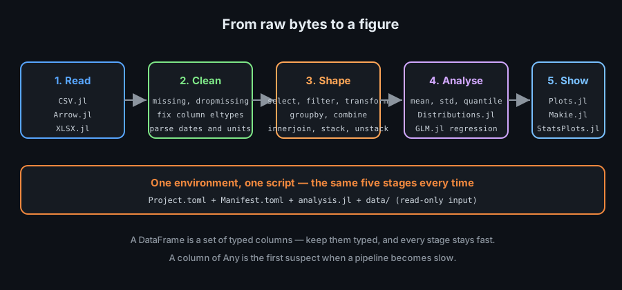
The workflow has five stages, and every stage has a well-chosen tool: read the bytes, clean the table, reshape it, compute statistics, draw the result. What separates a good analysis from a lucky one is that each stage is written down and can be re-run on next month's file without editing anything.
Tabular Data with DataFrames
A DataFrame is a collection of equal-length, separately typed columns with names. That one design decision explains almost all of its behaviour: fast per-column operations, type stability per column, and no per-cell parsing.
Building and Inspecting a DataFrame
Start by looking at your data before doing anything to it. Structure first, statistics later.
using DataFrames

# From column vectors — the usual way
df = DataFrame(
    id    = 1:4,
    name  = ["Ada", "Grace", "Alan", "Edsger"],
    score = [91.0, 88.5, 95.0, 79.5],
    pass  = [true, true, true, false],
)

# Inspect before you analyse
size(df)                 # (4, 4)      rows, columns
names(df)                # column names, in order
eltype.(eachcol(df))     # the TYPE of every column — the key diagnostic
first(df, 2)             # the first two rows
df[!, :score]            # a column without copying
describe(df)             # count, mean, min, max, std per numeric column

# Row access: integer row plus column name
df[3, :name]             # "Alan"

# Column order and additions
select!(df, :id, :name)                 # keep only these two
df.passed = df.score .>= 80             # add a computed column
rename!(df, :passed => :ok)

# Column types are fixed at creation: a column cannot mix Int and String.
# To hold mixed values, the column's type becomes Any or Union{...} —
# which is the first thing to look for when a DataFrame is slow.
The eltype.(eachcol(df)) line is worth running on every new dataset. A column you expect to be Float64 but that reports Any will make every later operation slower and every plot stranger.
Selecting and Filtering
The @select/@filter macros (from DataFramesMeta.jl) and the plain function forms express the same intent; knowing the plain form first removes the mystery.
using DataFrames

# select: choose and compute
select(df, :name, :score)
select(df, :name, :score, :score => (s -> s .* 1.1) => :adjusted)
select(df, Not(:id))                     # everything except id
select(df, r"^s")                        # columns matching a pattern
select(df, All()).score                   # a single column as a vector

# filter: keep rows that satisfy a condition
filter(:score => >(80), df)
filter(row -> row.pass && row.score > 90, df)
filter([:score, :pass] => (s, p) -> s > 90 && p, df)   # several columns at once

# subset with @subset semantics, but as a function
subset(df, :score => ByRow(>(80)), :pass => ByRow(identity))

# Sort, on one or several columns
sort(df, :score)
sort(df, [:pass, :score], rev = [false, true])   # pass first, then score down

# Chaining reads inside-out; `|>` makes it readable left-to-right
result = df |>
    x -> filter(:pass => identity, x) |>
    x -> select(x, :name, :score) |>
    x -> sort(x, :score, rev = true)
Filtering by column name (:score => >(80)) is both faster and clearer than filtering by row object, because it tells the compiler which columns the predicate needs. Reach for the row form only when the condition genuinely spans columns.
Transforming Columns
A transformation is a column expression: source columns, a function, and a new name. Once that pattern clicks, most wrangling becomes one line.
using DataFrames

# The general form:  :source(s) => function => :newname
transform(df,
    :score            => (s -> s ./ maximum(s))          => :relative,
    :name             => (n -> uppercase.(n))            => :name_upper,
    [:score, :pass]   => ((s, p) -> s .* p)              => :earned,
)

# transform keeps all existing columns; select keeps only the ones you name
select(df, :id, :score => ByRow(round) => :score_rounded)

# Broadcasting works directly on columns — no apply() needed
df.percentile = (df.score .- minimum(df.score)) ./
                (maximum(df.score) - minimum(df.score)) .* 100

# Rows to columns and back
transform(df, AsTable([:score]) => ByRow(sum) => :total)

# Delete a column
select!(df, Not(:total))

# Working with a copy vs in place: functions ending in `!` mutate.
df2 = transform(df, :score => ByRow(sqrt) => :root)    # df unchanged
transform!(df, :score => ByRow(sqrt) => :root)         # df changed
The bang convention from earlier chapters carries the same meaning here: a function ending in ! mutates its first argument. In an analysis script, prefer the non-mutating form until the data is large enough that copying matters.
Reading and Writing Data
Most datasets arrive as text. Parsing them correctly — and recording what the parse did to your types — is the least glamorous and most consequential part of the job.
CSV Files
CSV.jl parses to a DataFrame in one call, and its options are worth reading once because they decide your column types.
using CSV, DataFrames

# Read with inference — the everyday case
df = CSV.read("sales.csv", DataFrame)

# Read with intent: say what each column means
df = CSV.read("sales.csv", DataFrame;
    delim            = ',',
    header           = 1,
    missingstring    = ["", "NA", "NULL", "-"],   # all the spellings you have seen
    types            = Dict("id" => Int, "date" => Date, "revenue" => Float64),
    dateformat       = dateformat"yyyy-mm-dd",
    pool             = true,      # strings become pooled: memory wins on repeats
)

# Only the columns you need — much faster on wide files
CSV.read("sales.csv", DataFrame; select = ["date", "revenue", "region"])

# Peek at a huge file without loading it
CSV.read("huge.csv", DataFrame; limit = 100)

# Write it back
CSV.write("clean.csv", df; delim = ',')

# Common failure: a column of numbers with one "n/a" in it.
# Inference then produces a Union or String column, and totals break later.
# Fix it at read time with `missingstring` or `types`, not afterwards.
The last note is the recurring lesson of this chapter: type decisions happen at the boundary. Repairing a column after it has been read as String means parsing it again, in code that nobody will remember to run.
Other Formats
CSV is the interchange format; Arrow is the fast one; Parquet is the durable columnar one. Knowing when to use each saves real time.
using Arrow, DataFrames

# Arrow: zero-copy friendly, ideal between processes
Arrow.write("data.arrow", df)
df2 = DataFrame(Arrow.Table("data.arrow"))

# Parquet: columnar, compressed, the warehouse standard
using Parquet2
Parquet2.writefile("data.parquet", df)
df3 = DataFrame(Parquet2.Dataset("data.parquet"))

# Excel, when the file really is a spreadsheet
using XLSX
xf = XLSX.readxlsx("book.xlsx")
sheetnames(xf)                        # which sheets exist
df4 = DataFrame(XLSX.gettable(xf["Sheet1"]))

# Databases and remote sources
using SQLite
db = SQLite.DB("local.db")
df5 = DataFrame(DBInterface.execute(db, "SELECT * FROM sales WHERE revenue > 0"))

# Rule of thumb:
#   CSV      → humans, git, small files, interchange
#   Arrow    → fast intermediate steps inside one pipeline
#   Parquet  → large, long-lived, read column subsets
The choice matters at scale and barely at all for the four-row examples in this lesson. Pick CSV for anything a person must read; pick Arrow or Parquet when the file becomes the bottleneck.
Missing Data
missing is a value, not an error. Every function in Julia either propagates it — 1 + missing is missing — or refuses it explicitly. That is the design that keeps analyses honest.
using DataFrames, Statistics

# A missing value propagates rather than silently becoming zero
1 + missing                 # missing
mean([1.0, missing, 3.0])   # missing — the honest answer

# Decide explicitly what to do
mean(skipmissing([1.0, missing, 3.0]))    # 2.0
count(ismissing, df.score)                # how many are missing?
df.score = coalesce.(df.score, 0.0)       # replace with a default, consciously

# Column operations handle missing by default
describe(df)                # count of non-missing, then statistics

# Drop or keep rows with missing values
dropmissing(df)                          # rows where ANY column is missing
dropmissing(df, :revenue)                # only where revenue is missing
completecases(df)                        # a Bool vector: which rows are complete

# Subsetting with missing needs care: missing is not false
filter(:score => >(80), df)              # keeps only rows where the test is TRUE
subset(df, :score => ByRow(x -> !ismissing(x) && x > 80))

# Union types describe "Float64 or missing" precisely
typeof(df.score)            # Vector{Union{Missing, Float64}}
The subsetting rule is the one that causes silent data loss: a predicate that returns missing is treated as "does not match", so rows with unknown values vanish from a filtered result. Filter them deliberately, and print the count before and after.
Grouping, Joining and Reshaping
Most analysis is the same three moves applied to tables: split them into groups, combine each group into a summary, and attach related columns from another table.
Split, Apply, Combine
groupby does not copy data — it records which rows belong to which group. combine then produces one row per group.
using DataFrames, Statistics

# groupby + combine: one output row per group
gdf = groupby(df, :region)

combine(gdf,
    :revenue => sum                       => :total,
    :revenue => mean                      => :average,
    :revenue => (r -> maximum(r) - minimum(r)) => :spread,
    nrow                                  => :orders,      # how many rows per group
)

# Group by several columns at once
combine(groupby(df, [:region, :quarter]), :revenue => sum => :total)

# Keep every original row and broadcast the group summary back onto it
transform(gdf, :revenue => sum => :region_total)
transform(gdf, :revenue => (r -> r ./ sum(r)) => :share_of_region)

# Iterate groups directly when the computation is not row-shaped
for (key, sub) in pairs(gdf)
    println(key.region, ": ", nrow(sub), " rows")
end

# A single group is returned as a NamedTuple of columns with . and .:
combine(groupby(df, :region), :revenue => mean)
The distinction between combine and transform is the one to hold on to: use combine when the answer is one row per group, and transform when each original row needs a value that depends on its group.
Joins
Two tables describe more than either alone. A join is the operation that puts them back together, and the kind decides what happens to unmatched rows.
using DataFrames

customers = DataFrame(id = [1, 2, 3], name = ["Ada", "Grace", "Alan"])
orders    = DataFrame(id = [2, 2, 3, 4], amount = [10.0, 5.0, 7.0, 1.0])

# Inner join: only ids present in both (4 is dropped, 1 is dropped)
innerjoin(orders, customers, on = :id)

# Left join: keep every order, fill unmatched customer names with missing
leftjoin(orders, customers, on = :id)

# Right join: keep every customer, including those with no orders
rightjoin(orders, customers, on = :id)

# Outer join: everything from both, missing where the other side is absent
outerjoin(orders, customers, on = :id)

# Different column names on each side
leftjoin(orders, customers, on = :id => :customer_id)

# Several key columns
leftjoin(a, b, on = [:id, :date])

# Make the unmatched rows visible on purpose — the diagnostic habit:
nrow(orders) == nrow(innerjoin(orders, customers, on = :id)) ||
    @warn "some orders have no matching customer"
Duplicate keys are the classic silent surprise in joins: four orders matched to two customers becomes four rows, which is correct, but a summary taken afterwards no longer counts orders the way the first table did. Check nrow after every join.
Reshaping
Wide tables are for reading, long tables are for plotting and modelling. stack and unstack convert between the two.
using DataFrames

wide = DataFrame(country = ["RO", "FR"], y2024 = [10, 20], y2025 = [12, 21])

# wide → long: one row per (country, variable) pair
long = stack(wide, [:y2024, :y2025]; variable_name = :year, value_name = :visits)
#   country  year    visits
#   RO       y2024   10
#   FR       y2024   20
#   RO       y2025   12
#   FR       y2025   21

# long → wide: one column per distinct value of `year`
unstack(long, :country, :year, :visits)

# Reshaping is what makes plotting simple: the long form maps
# directly onto x, y, and colour aesthetics.
Reshaping pays for itself the first time a plot needs a legend: a long table gives the plotting library one call, while the wide form makes you write a loop of series with hand-made labels.
Statistics and Modelling
Julia's statistics are ordinary functions in the Statistics standard library and in Distributions.jl. Nothing here needs a data-frame-shaped special case.
Descriptive Statistics
Description first: the shape of a distribution tells you whether the fancy method you planned is appropriate.
using Statistics, StatsBase

x = [12.0, 15.0, 15.0, 18.0, 21.0, 15.0, 300.0]     # note the outlier

mean(x)          # 56.6   — dragged by the outlier
median(x)        # 15.0   — robust
std(x)           # sample standard deviation
var(x)           # variance
quantile(x, [0.25, 0.5, 0.75])      # the quartiles
iqr(x)           # interquartile range
mode(x)          # most frequent value
extrema(x)       # (min, max)
cor(x, y)        # Pearson correlation
cov(x, y)        # covariance

# Summaries with more context
using StatsBase
describe(x)                       # count, mean, min, quartiles, max
skewness(x)                       # asymmetry
kurtosis(x)                       # tail weight

# For a vector containing missing values, use the skip variant
mean(skipmissing(x))
median(skipmissing(x))

# Weighted form
mean(x, weights(1:length(x)))
The mean/median pair in this example is the whole argument for looking before you test: one entry at 300 changes the mean by a factor of four and the median not at all. Any conclusion drawn from the mean alone would be wrong.
Distributions and Hypothesis Tests
Distributions.jl gives you the same interfaces for every distribution — density, cumulative, quantile, sampling — so code written once works on all of them.
using Distributions, HypothesisTests

# Fit a distribution to data
d = fit(Normal, x)                 # Normal(μ = 56.6, σ = 107.9)
mean(d); std(d)
fit(Gamma, filter(>(0), x))

# The four universal functions
pdf(d, 15.0)          # density at a point
cdf(d, 15.0)          # P(X <= 15)
quantile(d, 0.95)     # the 95th percentile
rand(d, 5)            # five samples
rand(MersenneTwister(1), d, 5)     # reproducible samples

# Confidence intervals
using StatsBase
ci = mean(x) ± 1.96 * std(x) / sqrt(length(x))
ci

# Hypothesis tests
OneSampleTTest(x, 15.0)            # is the mean different from 15?
EqualVarianceTTest(a, b)           # two sample means
ChisqTest(counts)                  # independence in a contingency table
pvalue(OneSampleTTest(x, 15.0))    # no evidence against the null here

# The rule that saves careers: decide the test BEFORE looking at p-values,
# and report the effect size, not only the significance.
The last comment is not decoration. With enough data, a difference of no practical importance becomes statistically significant; the test answers "could this be chance?", not "does this matter?".
Regression with GLM
GLM.jl fits linear and generalized linear models with R-style formulas, and it returns a table of coefficients you can read directly.
using GLM, DataFrames

df = DataFrame(y = [2.1, 4.2, 6.1, 8.3, 10.2],
               x = [1.0, 2.0, 3.0, 4.0, 5.0],
               g = ["a", "a", "b", "b", "b"])

# Formula interface: response ~ predictors (categoricals auto-expand)
model = lm(@formula(y ~ x + g), df)
coef(model)                 # coefficients
coeftable(model)            # estimate, std error, t-statistic, p-value
r2(model)                   # how much variance is explained
predict(model, df)          # fitted values
residuals(model)            # check these: shape matters more than R²

# A logit model on binary data
logit_model = glm(@formula(pass ~ score), df, Binomial(), LogitLink())
odds_ratio(logit_model)

# With missing values, drop the affected rows explicitly first
clean = dropmissing(df, [:y, :x])
lm(@formula(y ~ x), clean)

# Diagnostics worth running before believing a coefficient
using Statistics
std(residuals(model))                 # residual scale
cor(predict(model, df), df.y)^2       # sanity check against r2
Plotting
A figure is an argument. The plotting library you choose decides how much of that argument you express in code and how much in your head.
The Plotting Ecosystem
Julia has two families and a wrapper. Knowing what each is for prevents the usual week spent comparing benchmarks.
| Package | What it is | Use it for |
|---|---|---|
| Plots.jl | A unified API over many backends (GR, PyPlot, Plotly) | Everyday figures, quick iteration, publication PDFs |
| Makie.jl | A native Julia graphics system with GPU backends | Interactive, animated, very large datasets |
| StatsPlots.jl | Statistical recipes for Plots.jl | Histograms, boxplots, violin plots, group comparisons |
| VegaLite.jl | Grammar-of-graphics, JSON output | Web-embedded charts, explicit encodings |
Start with Plots.jl: its API is stable, its defaults are readable, and it changes backend with one call. Move to Makie when you need interactivity or animations, not because it renders an extra frame per second.
Plots and Makie in Practice
The same figure in both families shows the trade-off clearly: Plots.jl is terse, Makie is explicit.
using Plots
default(titlefontsize = 12, legend = :topleft)

# A line plot with two series
plot(1:10, (1:10).^2; label = "square", lw = 2)
plot!(1:10, (1:10).^3; label = "cube", lw = 2, ls = :dash)
xlabel!("n"); ylabel!("value"); title!("Growth")
savefig("growth.pdf")

# Scatter with a colour dimension
scatter(df.x, df.y; zcolor = df.score, markersize = 4, colorbar = true)

# Several subplots in one figure
p1 = plot(1:10, rand(10); title = "A")
p2 = histogram(randn(1000); title = "B")
plot(p1, p2; layout = (1, 2), size = (800, 300))

# The same picture in Makie, interactively
using CairoMakie
f = Figure()
ax = Axis(f[1, 1]; xlabel = "n", ylabel = "value", title = "Growth")
lines!(ax, 1:10, (1:10).^2; label = "square")
lines!(ax, 1:10, (1:10).^3; label = "cube", linestyle = :dash)
axislegend(ax)
save("growth.png", f)

# Choosing: Plots.jl for scripts and documents, Makie for exploration you
# look at while it runs, or for figures with thousands of marks.
Saving to a vector format (.pdf, .svg) is the right default for anything that will be printed or scaled; use .png for screens and quick feedback.
Statistical Plots
Statistical plots answer specific questions — spread, distribution, relationship — and each has a standard form that readers already know how to interpret.
using StatsPlots, DataFrames

# Distribution of one variable
histogram(df.score; bins = 20, normalize = :pdf, legend = false)
density(df.score; fill = (0, 0.5, :blue))

# Distribution by group: boxplot is the standard comparison
boxplot(string.(df.pass), df.score; xlabel = "pass", ylabel = "score")
violin(string.(df.pass), df.score; show_median = true)

# Relationship between two variables with a fitted line
scatter(df.x, df.y; label = "data")
abline!(coef(lm(@formula(y ~ x), df)); label = "fit")

# A correlation matrix as a heatmap
using Statistics
C = cor(Matrix(select(df, :x, :y)))
heatmap(C; c = :balance, annotate = true)

# Time series with a rolling mean
plot(df.date, df.value; label = "raw", alpha = 0.4)
plot!(df.date, rolling(mean, df.value, 7); label = "7-day mean", lw = 2)

# Saving a figure at a size that survives review
savefig("comparison.pdf"; size = (900, 600))
One habit makes figures trustworthy: plot before and after every data transformation, not only at the end. A join that silently multiplied rows is obvious in a scatter plot and invisible in a summary table.
A Reproducible Analysis Workflow
The difference between an analysis and an anecdote is whether somebody else can run it. Everything below serves that single goal.
Reproducible Analysis
Three things must be recorded: the environment, the code, and the data's identity. Miss any one and the result is a story rather than a result.
# 1. The environment — committed, not described
#    ] activate .
#    ] add DataFrames CSV Statistics Plots GLM
#    git add Project.toml Manifest.toml

# 2. The code — one script that runs from raw data to figures
# analysis/
#   Project.toml
#   Manifest.toml
#   main.jl            # the whole pipeline, in stages
#   src/clean.jl       # one function per stage
#   src/analyse.jl
#   figures/           # written by the script, never edited by hand
#   data/raw/          # read-only inputs, with a checksum
#   data/processed/    # intermediate results, recreatable

# 3. The data's identity — a hash, so you know which version produced the figure
using SHA
bytes2hex(sha256(read("data/raw/sales.csv")))     # record this in the report

# Make randomness reproducible too
using Random
rng = MersenneTwister(20260912)
sample(df, 1000; replace = false)
The checksum line is small and consequential: when two people get different numbers from "the same file", the hash settles it in one command.
Scripts, Functions and Notebooks
Notebooks are excellent for exploring and poor for repeating. Convert anything worth keeping into a function in a script.
# main.jl — the pipeline, readable at a glance
using Pkg; Pkg.activate(@__DIR__)

include("src/clean.jl")
include("src/analyse.jl")

function main()
    raw   = load_raw("data/raw/sales.csv")
    clean = clean_sales(raw)                 # every stage is a function
    stats = summarise(clean)
    write_figures(clean, "figures/")
    write_table(stats, "data/processed/summary.csv")
    @info "pipeline complete" rows = nrow(clean)
end

main()      # one entry point:  julia --project=. main.jl

# Rules that keep the pipeline maintainable
#   - functions, not top-level scripts with side effects
#   - the raw data directory is never written to
#   - every figure is regenerated by the script, never edited afterwards
#   - stage boundaries print the row count, so a bad join is visible

using Test
@testset "clean_sales" begin
    raw = DataFrame(id = [1], revenue = ["10"], region = ["RO"])
    out = clean_sales(raw)
    @test eltype(out.revenue) == Float64      # the type contract holds
    @test nrow(out) == 1                      # no rows lost
end
The row-count print is the cheapest safeguard in data work. A join, a dropmissing, or a filter that changes the count by more than expected is exactly the bug that survives every test you did not write.
Common Pitfalls
These are the errors that produce a confident, wrong number.
| Pitfall | Consequence | Fix |
|---|---|---|
Column typed Any or String after a messy read | Amounts sort and sum as text | Fix types at read time with types and missingstring |
Filtering a column that contains missing | Rows silently disappear | subset with an explicit !ismissing check |
| Join that duplicates rows | Totals inflate with no warning | Compare nrow before and after; deduplicate keys |
describe on the whole frame only | Group differences stay invisible | combine(groupby(df, :group), ...) |
| Mean reported for a skewed variable | A number no individual has | Report median and quartiles as well |
| Unseeded sampling | The sample cannot be reproduced | MersenneTwister(seed) |
| Editing figures by hand | Figure and code disagree | Regenerate; never touch the output file |
| Quoting a point estimate only | Uncertainty disappears from the report | Report the interval, not only the mean |
A data pipeline is judged by its second run: the one done by somebody else, on next month's file, without you in the room.
DataFrame is typed columns with names, so column types — not row loops — decide performance. Read CSVs with explicit types and missingstring, treat missing as a value to handle deliberately, and remember that missing inside a predicate silently drops rows. Shape tables with select, filter, transform, groupby+combine, joins, stack and unstack, checking nrow across every join. Use Statistics, Distributions, HypothesisTests and GLM for analysis, and always inspect residuals before trusting a coefficient. Draw figures with Plots.jl or Makie, and wrap the chain in an activated environment, one entry-point script, and a data checksum.
Next, take the same habits into simulation and modelling: Scientific Computing with SciML.