
Scientific Computing
DifferentialEquations.jl suite — roughly the differential-equation solver of the whole language — started a family now known as SciML: modelling, solving, fitting, and simulating physical systems with automatic differentiation and GPU support wired in. This lesson covers the part you need to be productive: state the model, pick a solver, simulate, and keep the units and precision honest.
The examples are deliberately small — a harmonic oscillator, an epidemiological SIR model, a diffusion equation — but the workflow scales unchanged to thousands of state variables. What changes at scale is not the API; it is the attention you pay to Jacobian structure, sparse storage, and solver stiffness. Those are the subjects of this page.
The examples are deliberately small — a harmonic oscillator, an epidemiological SIR model, a diffusion equation — but the workflow scales unchanged to thousands of state variables. What changes at scale is not the API; it is the attention you pay to Jacobian structure, sparse storage, and solver stiffness. Those are the subjects of this page.
The SciML Ecosystem
SciML is not one package. It is a set of composable packages that share a single interface, so the solver you pick is independent of the way you write the model.
What SciML Covers
Four kinds of work, one toolkit: state a model, solve it, fit it to data, and differentiate through it.
| Package | Which problem | Typical call |
|---|---|---|
| DifferentialEquations.jl | ODEs, SDEs, DAEs, DDEs, PDE discretisations | solve(ODEProblem(...), Tsit5()) |
| ModelingToolkit.jl | Symbolic model definition and simplification | ODEProblem(sys, u0, tspan, p) |
| Optimization.jl | Parameter fitting, inverse problems | solve(OptimizationProblem(...)) |
| SciMLSensitivity.jl | Gradients through a solver | Zygote.gradient over solve |
| LinearSolve.jl | The linear system inside every implicit step | solve(LinearProblem(A, b)) |
The value of the shared interface is that these compose: a symbolically defined model, solved by an implicit method, differentiated for a parameter fit, and run on a GPU — without rewriting the model between stages.
ModelingToolkit and Symbolic Models
ModelingToolkit.jl lets you write the equations and have Julia do the algebra: build the Jacobian symbolically, simplify, and generate fast code from it.
using ModelingToolkit
using ModelingToolkit: t_nounits as t, D_nounits as D

# Parameters and variables
@parameters k c
@variables x(t) v(t)

# The system, written as equations — no manual Jacobian, no manual sorting
eqs = [D(x) ~ v,
       D(v) ~ -k * x - c * v]

@named oscillator = ODESystem(eqs, t)

# Optionally simplify before compiling
sys = structural_simplify(oscillator)

# Build the problem and solve it exactly like a hand-written one
using DifferentialEquations
u0 = [x => 1.0, v => 0.0]
p  = [k => 4.0, c => 0.2]
prob = ODEProblem(sys, u0, (0.0, 20.0), p)
sol  = solve(prob, Tsit5())

# What you gain over the hand-written form:
#   - the Jacobian is derived symbolically and stays correct after edits
#   - stiff and implicit solvers get a sparse or banded Jacobian for free
#   - the same equations can be exported to other languages if needed
The gain is not convenience for its own sake. A hand-written Jacobian that drifts from the hand-written equations produces a solver that converges more slowly every time the model changes — and eventually fails to converge at all.
Choosing the Approach
Three ways to define a model, three appropriate situations. Pick the simplest one that fits the work.
# 1. Out-of-place function: clearest, fine for small systems (< 100 states)
function f(u, p, t)
    x, v = u
    k, c = p
    return [v, -k * x - c * v]
end

# 2. In-place function: no allocation per step — the right default for
#    anything large or performance-sensitive
function f!(du, u, p, t)
    x, v = u[1], u[2]
    k, c = p[1], p[2]
    du[1] = v
    du[2] = -k * x - c * v
    return nothing
end

# 3. Symbolic system: the equations are the source of truth
#    (see ModelingToolkit above)

# Rules of thumb:
#   small system, iterating on the maths   → out-of-place, arrays
#   large system, timing matters           → in-place, StaticArrays for < 30 dims
#   many parameters to fit, stiff system   → symbolic, for the Jacobian
#   state is naturally a struct            → any of the three, via parameters
For systems under about thirty dimensions, SVector from StaticArrays.jl is often the single largest speed-up available, because the state lives on the stack instead of the heap and the compiler can unroll the whole right-hand side.
Differential Equations
Solving an ODE in Julia is three steps: write the derivative, wrap it in a problem, and hand it to a solver. The fourth step — choosing the solver — is where the science is.
Defining an ODE Problem
The standard form is the SIR epidemic model: three coupled first-order equations, one parameter set, one initial state.
using DifferentialEquations

# SIR: susceptible, infected, recovered, with transmission β and recovery γ
function sir!(du, u, p, t)
    S, I, R = u                  # state
    β, γ    = p                  # parameters
    N = S + I + R                # total population (assumed constant)
    du[1] = -β * S * I / N       # new infections leave the susceptible pool
    du[2] =  β * S * I / N - γ * I
    du[3] =  γ * I
    nothing
end

u0 = [990.0, 10.0, 0.0]          # one infected person in a town of 1000
tspan = (0.0, 100.0)
p = [0.3, 0.1]                   # β, γ  → basic reproduction number R₀ = β/γ = 3

prob = ODEProblem(sir!, u0, tspan, p)
sol  = solve(prob, Tsit5())

sol.t                            # the time points the solver chose
sol.u[end]                       # the final state
sol[2, :]                        # the infected curve, all time points
sol(50.0)                        # interpolate at t = 50
Two details repay attention. R₀ = β/γ is the number every epidemiological conclusion hangs on, and it is a property of the parameters, not of the solver. And the in-place form sir! writes into du without allocating — which is what makes a thousand-parameter sweep affordable.
Solving and Plotting
The solution object behaves like a function, so plotting is a one-liner and any quantity you can compute from the state is available at any time.
using Plots

# The ready-made recipe: one line per state variable
plot(sol; labels = ["Susceptible" "Infected" "Recovered"],
     xlabel = "days", ylabel = "people", lw = 2)

# Derived quantities at any time, including interpolated points
ts = range(0, 100; length = 200)
infected = [sol(t)[2] for t in ts]                # dense interpolation
plot(ts, infected; label = "infected", xlabel = "days")

# Peak infection and when it happens — the quantity policy cares about
peak   = maximum(sol[2, :])
t_peak = sol.t[argmax(sol[2, :])]
@info "epidemic peak" infected = round(peak) day = round(t_peak)

# Choose output points explicitly when you need a regular grid
sol2 = solve(prob, Tsit5(); saveat = 0.5)         # every half day

# Ensemble runs: many parameter sets, in parallel threads
function make_prob(β)
    ODEProblem(sir!, u0, tspan, [β, 0.1])
end
ensemble = EnsembleProblem(make_prob(0.2:0.05:0.5))
sols = solve(ensemble, Tsit5(); trajectories = 7)  # one run per β
plot(sols; legend = false, xlabel = "days", ylabel = "I")
The ensemble pattern is the reason to learn EnsembleProblem early: parameter sweeps, Monte-Carlo uncertainty, and multi-start fits are all the same idea, and the thread-parallel form costs one extra argument.
Stiff Systems and Solver Choice
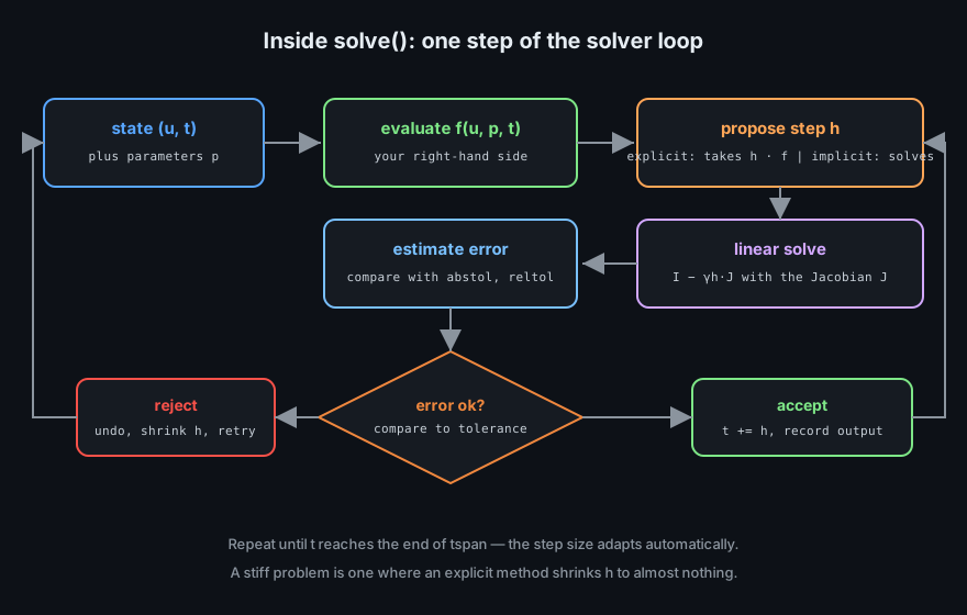
A stiff system has components that change on wildly different timescales. Choosing a non-stiff solver for a stiff problem produces a run that seems to hang rather than fail.
# Explicit methods (Tsit5, Vern7): cheap per step, but the step size is
# limited by the FASTEST timescale in the system.
solve(prob, Tsit5())

# Implicit methods (Rodas5, FBDF, Rosenbrock23) solve a linear system per
# step instead: more work per step, far fewer steps on a stiff problem.
solve(prob, Rodas5())

# Let the library guess — a good default while prototyping
solve(prob, AutoTsit5(Rosenbrock23()))

# How to tell that a problem is stiff:
#   - Tsit5 takes tens of thousands of steps for a smooth-looking curve
#   - the step size collapses to something tiny after an initial phase
#   - a chemical or biological system whose rate constants differ by 1e3+

# Options that matter for stiff problems
solve(prob, Rodas5();
    jac      = true,               # use an analytically or symbolically derived Jacobian
    autodiff = true,               # or let Julia differentiate the right-hand side
    abstol   = 1e-10,              # tolerances decide the step size — set them deliberately
    reltol   = 1e-8,
    saveat   = 0.1,
)

# A check before trusting any solution
sol.retcode == ReturnCode.Success || @error "solve failed" sol.retcode
Two diagnostics tell you the solver is wrong for the problem: the step count (sol.stats.nsteps) far exceeds what the smoothness suggests, and the tolerance you set is not the accuracy you got. Tightening tolerances means more steps, not automatically a better answer.
Beyond ODEs
One interface solves much more than ordinary differential equations. The state vector changes meaning, and the rest of your code stays the same.
PDEs by the Method of Lines
A partial differential equation is turned into a large ODE system by discretising space and keeping time continuous — the method of lines.
using DifferentialEquations, LinearAlgebra

# Heat equation:  ∂u/∂t = D ∂²u/∂x²  on [0, 1] with u = 0 at both ends.
# Discretise x into N interior points; the second derivative becomes
# neighbouring-point differences, i.e. a tridiagonal matrix.

function heat!(du, u, p, t)
    D, dx, N = p
    for i in 1:N
        left  = i == 1 ? 0.0 : u[i-1]      # the boundary value
        right = i == N ? 0.0 : u[i+1]
        du[i] = D * (left - 2u[i] + right) / dx^2
    end
    nothing
end

N  = 100
dx = 1 / (N + 1)
u0 = [sin(pi * i * dx) for i in 1:N]        # a smooth initial profile
p  = (0.01, dx, N)

prob = ODEProblem(heat!, u0, (0.0, 10.0), p)

# The result is a matrix: rows are space, columns are time
sol = solve(prob, Rodas5(); saveat = 0.25)
heatmap(sol.t, range(dx, 1-dx; length = N), sol';
        xlabel = "time", ylabel = "space", title = "heat diffusion")

# Notes that matter at scale:
#   - use a MATRIX-free or sparse Jacobian; a dense N×N matrix is waste
#   - the loop is allocation-free, so millions of steps stay cheap
#   - explicit methods need dt < dx²/(2D) — stiff solvers do not
The stability condition in the last comment is the reason implicit solvers dominate PDE work: refining the spatial grid by ten squares the number of points but shrinks the stable explicit step by a hundred. An implicit method pays a linear solve per step to escape that constraint entirely.
Discrete and Stochastic Models
Not every system is continuous. Julia has dedicated problem types for jumps, noise, and delays, and they share the same solve call.
using DifferentialEquations, StochasticDiffEq, DiffEqJump

# 1. SDE: an ODE with noise — geometric Brownian motion
function gbm!(du, u, p, t)
    μ, σ = p
    du[1] = μ * u[1]              # drift
    nothing
end
function gbm_noise!(du, u, p, t)
    μ, σ = p
    du[1] = σ * u[1]              # diffusion term
    nothing
end
prob_sde = SDEProblem(gbm!, gbm_noise!, [100.0], (0.0, 1.0), (0.1, 0.3))
sol_sde  = solve(prob_sde, EM(); dt = 1e-3)

# 2. Discrete jumps: a chemical or population process
rate(u, p, t) = 0.5 * u[1]                     # exponential decay of counts
affect!(integrator) = integrator.u[1] -= 1
jump = ConstantRateJump(rate, affect!)
prob_jump = DiscreteProblem([50], (0.0, 20.0))
sol_jump  = solve(JumpProblem(prob_jump, jump), SSAStepper())

# 3. Delay differential equations: the derivative depends on a past value
function dde!(du, u, h, p, t)
    du[1] = -p * h(p, t - 1.0)[1]              # depends on 1 unit ago
    nothing
end
prob_dde = DDEProblem(dde!, [1.0], (u, p, t) -> [1.0], (0.0, 10.0), 1.0)

# Every one of them returns a solution you can plot and index the same way.
Three different mathematics, one calling convention. That consistency is the practical argument for SciML: expertise in one problem type transfers directly to the next.
Events: When the State Changes the Rules
Many models change behaviour at a threshold — a ball hits the floor, a drug is re-dosed, a valve closes. An event callback is how that is expressed.
using DifferentialEquations

# A bouncing ball: reverse the velocity when height crosses zero
function ball!(du, u, p, t)
    du[1] = u[2]              # height
    du[2] = -9.81             # velocity (gravity)
    nothing
end

# The event: trigger when height == 0, and reverse the velocity
function hit_floor!(integrator)
    integrator.u[2] = -0.9 * integrator.u[2]     # 0.9 = coefficient of restitution
    nothing
end
cb = ContinuousCallback(
    (u, t, integrator) -> u[1],                  # the condition
    hit_floor!;                                  # what to do when it fires
    affect_neg! = nothing,                       # crossing upwards: ignore
)

prob = ODEProblem(ball!, [10.0, 0.0], (0.0, 20.0))
sol  = solve(prob, Tsit5(); callback = cb)       # the solver handles the bounce

# Other event kinds
#   DiscreteCallback   → trigger on a schedule or from an external signal
#   terminate!()       → stop the integration when a condition is met
#   PresetTimeCallback → dose at t = 0, 8, 16, ...

# Rules for events
#   - keep the callback cheap: it runs inside the solver loop
#   - mutating `integrator.u` is the supported way to change the state
#   - the condition must change sign at the crossing, not merely touch zero
The last rule explains most event bugs: a condition like "distance to a target is less than ε" touches zero and bounces back without changing sign. Use a root-finding formulation — a quantity that crosses zero — and the solver will locate the moment accurately.
The last rule explains most event bugs: a condition like "distance to a target is less than ε" touches zero and bounces back without changing sign. Use a root-finding formulation — a quantity that crosses zero — and the solver will locate the moment accurately.
Linear Algebra for Simulation
Every implicit solver step ends in a linear system. That is why linear algebra decides whether a simulation finishes in a minute or a day.
Dense, Sparse and Structured Matrices
The choice of storage is the choice of algorithm. A matrix that is 99% zeros should never be stored as if it were full.
using LinearAlgebra, SparseArrays, LinearSolve

A = rand(1000, 1000)              # dense: 8 MB for Float64, O(n³) to factorise
x = A \ b                         # LU factorisation behind the backslash

# Sparse: store only the nonzeros
S = sprand(1000, 1000, 0.001)     # ~1000 nonzeros, a few kilobytes
S \ b                             # sparse LU, far faster than dense

# Build sparse matrices the way they are actually produced: from triplets
I = [1, 2, 3, 3]
J = [1, 2, 3, 1]
V = [10.0, 20.0, 30.0, 5.0]
T = sparse(I, J, V)               # duplicates are summed automatically

# Structured and banded matrices
using LinearAlgebra
D = Diagonal(1.0:1000.0)          # O(n) storage, O(n) solve
T2 = Tridiagonal(rand(999), rand(1000), rand(999))
B = Symmetric(rand(500, 500))

# Reuse a factorisation across many right-hand sides — the big win in a
# time loop where A is constant and only the unknown changes
F = lu(A)
F \ b1
F \ b2

# LinearSolve.jl unifies all backends behind one call
prob = LinearProblem(A, b)
sol  = solve(prob, LUFactorization())

# Rules of thumb
#   n < 100        → dense, no ceremony
#   banded/structured → use the structured type, get the free speed
#   sparse > 90% zeros → sparse; below that, dense is often faster
#   many solves, same matrix → factorise once, reuse
The "reuse the factorisation" note is the one that shows up in profiling most often. A simulation that re-factorises a constant matrix at every step does O(n³) work per step for no reason.
Eigenvalues and Factorisations
Stability analysis, modal decomposition, and least squares are all factorisations. Julia names them the way the mathematics does.
using LinearAlgebra

A = Symmetric(rand(5, 5))

# Eigen decomposition: A = V * Diagonal(λ) * V'
F = eigen(A)
F.values              # eigenvalues, ascending for a symmetric matrix
F.vectors             # columns are the eigenvectors
maximum(F.values) < 0 || @warn "unstable equilibrium: positive eigenvalue"

# For a non-symmetric matrix use eigen(A); for a generalised problem,
# eigen(A, B) solves A v = λ B v.

# Singular value decomposition: the workhorse of data and conditioning
U, S, V = svd(rand(10, 5))
S                     # singular values: min(S) small means ill-conditioned
cond(rand(10, 5))     # the condition number, made explicit

# Cholesky for symmetric positive-definite systems: twice as fast as LU
spd = A'A + I                       # guaranteed positive definite
L = cholesky(spd)
L \ b

# Least squares without normal equations
Q, R = qr(rand(100, 5))
F = qr(A)

# The stability check every simulation should print once
ρ = maximum(abs, eigvals(A))        # spectral radius
ρ < 1 || @warn "the iteration will not converge" ρ
The spectral-radius check is worth automating into a test: an explicit scheme whose update matrix has spectral radius at or above one will diverge, and it is far cheaper to catch that in a unit test than after a week-long run.
Iterative Solvers
When the matrix is huge and sparse, factorising it is not an option. Iterative methods solve it by repeated multiplication — often each step is the same right-hand-side evaluation your model already computes.
using LinearAlgebra, IterativeSolvers, SparseArrays

A = sprand(10_000, 10_000, 0.0001) + 10I     # sparse, well-conditioned
b = rand(10_000)

# Conjugate gradients: symmetric positive definite
x = cg(A, b; reltol = 1e-10, log = true)
x.iters                        # how many iterations were needed

# GMRES: general matrices
x2 = gmres(A, b; reltol = 1e-8, restart = 30)

# BiCGStab and MINRES for other structures
x3 = bicgstabl(A, b; reltol = 1e-8)

# Preconditioning is what makes these methods practical: transform the
# system so the iterative method converges in far fewer steps.
using Preconditioners
P = DiagonalPreconditioner(A)
x4 = cg(A, b; Pl = P, reltol = 1e-10)

# What goes wrong, and why
#   no convergence in `maxiter` → the matrix is ill-conditioned or the
#                                 preconditioner is wrong, not the tolerance
#   convergence slow for a PDE  → use a multigrid or incomplete-LU preconditioner
#   solution wrong but "converged" → check the residual: norm(A*x - b)

# Always verify:
norm(A * x - b) < 1e-8 || @error "the residual is too large" norm(A * x - b)
Verifying the residual is not optional. An iterative solver can stop for reasons that are not success — a zero right-hand side, a breakdown, a maximum iteration count — and the returned vector will look like any other solution.
Units, Precision and Speed
Numbers carry meaning beyond their value: a length of 3 is meaningless without a unit, and a Float64 is not exact. Julia lets you encode both facts in the type.
Quantities with Units
Unitful.jl makes the unit part of the type, so an equation that is dimensionally wrong fails to run — instead of silently producing a number in the wrong unit.
using Unitful

# Construct quantities explicitly
distance = 100u"m"
time     = 9.58u"s"
speed    = distance / time                 # 10.43 m/s — units divide like algebra

# Units are checked at run time, and errors are clear
#   distance + 5u"s"     → ERROR: DimensionError
#   velocity - distance  → ERROR: DimensionError

# Convert deliberately
ustrip(distance)                            # 100, with the unit stripped
convert(typeof(1.0u"km"), distance)         # 0.1 km
uconvert(u"km", distance)                   # the idiomatic form

# Use them throughout a simulation, including inside the solver
using DifferentialEquations, Unitful
function project!(du, u, p, t)
    g = 9.81u"m/s^2"
    du[1] = u[2]                            # height in m
    du[2] = -g                              # acceleration in m/s²
    nothing
end
prob = ODEProblem(project!, [10.0u"m", 0.0u"m/s"], (0.0u"s", 2.0u"s"))
sol  = solve(prob, Tsit5())
sol.u[end]                                  # a quantity with a unit

# Units in a solver cost a little performance and repay it immediately
# in correctness: the classic "forgot to convert minutes to seconds" bug
# cannot be written.
Use units at the boundaries of a computation — model definition, input parsing, reporting — and consider stripping them inside the hottest inner loop if profiling shows the conversion matters.
Arbitrary Precision and Accurate Sums
Float64 has about 16 significant digits and loses precision in ways that matter for chaotic or ill-conditioned problems. Julia has types for both concerns.
using LinearAlgebra

# BigFloat: arbitrary precision, set as a global default
setprecision(BigFloat, 256) do
    x = BigFloat(2)
    sqrt(x)                    # 1.41421356237309504880168872420969807856967187537694...
end

# Rational numbers: exact arithmetic where it is appropriate
r = 1//3 + 1//6                # 1//2, exactly
float(r)                       # 0.5

# Multiple-dispatch alternatives from the ecosystem
using DoubleFloats            # ~32 digits, much faster than BigFloat
xf = Double64(2)
sqrt(xf)

# Who cares about precision? Let a numeric example show it:
sum_bad  = sum(1e16 + (1.0 for _ in 1:10^6) .- 1e16)   # loses the small terms
sum_good = sum(BigFloat, 1e16 + (1.0 for _ in 1:10^6) .- 1e16)

# Catastrophic cancellation and how to see it
a = 1e16; b = 1e16 + 1
a == b                          # true! the two numbers are the same Float64

# Use these tools selectively: BigFloat is slow, and most simulations
# do not need it. Reach for it when the answer is sensitive to rounding.
The 1e16 + 1 example is the one to remember. It is not a Julia bug: 16 digits is all a Float64 has, so adding one to a number of magnitude 1e16 rounds away entirely. Any algorithm that subtracts nearly equal large numbers needs either reordering or higher precision.
Static Arrays, Special Functions and SIMD
Once correctness is established, the performance levers that actually move scientific code are few and well documented.
using StaticArrays, LoopVectorization

# 1. StaticArrays: small fixed-size vectors live on the stack.
#    For a 3-vector inside a million-step loop this is often 5–20× faster.
function norm_sv(v::SVector{3,Float64})
    sqrt(v[1]^2 + v[2]^2 + v[3]^2)     # unrolled, no allocation, no bounds checks
end
v = SVector(1.0, 2.0, 3.0)
norm_sv(v)

# 2. SIMD-friendly loops with @turbo (LoopVectorization.jl)
function saxpy!(y, a, x)
    @turbo for i in eachindex(y)
        y[i] += a * x[i]
    end
    y
end

# 3. Special functions from SpecialFunctions.jl, exact and fast
using SpecialFunctions
gamma(5.0)          # 24.0
erf(1.0)            # 0.8427007929497149
loggamma(1000.0)    # works where gamma(1000.0) overflows

# 4. Measure before believing any of it
using BenchmarkTools
@btime norm_sv($v)
@btime sum(abs2, v)

# The order that matters: correctness → allocation → type stability →
# vectorisation. Optimising in the other order produces fast wrong answers.
The closing line is the discipline of this whole track. Every technique here multiplies speed and can also multiply a silent error: a @turbo loop over an aliased array, or an SVector indexing bug, is far harder to see than a slow loop.
A Research Workflow
Scientific code has one requirement that ordinary software does not: the result must be defensible — someone must be able to reproduce the figure in your paper two years from now.
Notebooks, Scripts and Package Structure
Use notebooks to explore and scripts to produce results. The conversion should happen the day a result matters.
# The structure that survives peer review
#   study/
#     Project.toml            # exact dependencies, pinned
#     Manifest.toml           # committed
#     src/model.jl            # the equations — no I/O, no plotting
#     src/solve.jl            # parameter sets, solver choice, tolerances
#     src/figures.jl          # one function per figure in the paper
#     scripts/run_all.jl      # regenerates every figure from scratch
#     test/runtests.jl        # unit tests plus the invariants
#     data/                   # inputs, with checksums recorded
#     results/                # outputs, regenerated, never edited

# scripts/run_all.jl
using Pkg; Pkg.activate(dirname(@__DIR__))
using Study

for figure in (Figure1(), Figure2(), Figure3())
    save_figure(figure, joinpath("results", name(figure)))
    @info "figure written" figure = name(figure)
end

# WHY THE SEPARATION MATTERS
#   src/model.jl must be testable without running a simulation
#   tolerances are part of the result — record them next to the figure
#   the notebook you explored in is not the record of the result
The most common failure in computational work is not a wrong equation; it is a figure that cannot be regenerated because a parameter was typed once into a notebook cell that no longer exists.
Making a Simulation Reproducible
Four things make a numerical result reproducible: the code, the environment, the parameters, and the random seed.
# Record everything that could change the number you report
struct RunConfig
    solver :: String
    abstol :: Float64
    reltol :: Float64
    seed   :: UInt64
    julia  :: String          # VERSION captured with the result
end

function run_study(cfg::RunConfig)
    rng  = MersenneTwister(cfg.seed)
    prob = build_problem(; rng)
    sol  = solve(prob, solver(; abstol = cfg.abstol, reltol = cfg.reltol))
    sol.retcode == ReturnCode.Success || error("solve failed: $(sol.retcode)")
    return summarise(sol), cfg
end

# Write the configuration next to the output, as machine-readable JSON
using JSON3
results, cfg = run_study(RunConfig("Rodas5", 1e-10, 1e-8, 20260912, string(VERSION)))
open("results/run.json", "w") do io
    JSON3.write(io, (cfg = cfg, results = results))
end

# The four questions a reviewer will ask:
#   which commit?      → git describe in the run record
#   which versions?    → Manifest.toml
#   which parameters?  → run.json
#   which random seed? → run.json
Writing the configuration beside the result turns a study from an anecdote into an artefact. It costs twenty lines and removes the entire class of "we cannot reproduce that figure" conversations.
Common Pitfalls
Each of these has produced a published correction at some point.
| Pitfall | Consequence | Fix |
|---|---|---|
| Non-stiff solver on a stiff problem | A run that appears to hang, or loses accuracy silently | Check sol.stats.nsteps; switch to Rodas5 or FBDF |
| Tolerances left at defaults | Reported accuracy unrelated to requested accuracy | Set abstol and reltol, and record them |
Not checking sol.retcode | A failed solve plotted as a result | Assert success before using the solution |
| Dense matrix for a sparse problem | O(n³) work and O(n²) memory for a banded system | SparseMatrixCSC, Tridiagonal, or a matrix-free operator |
| Iterative solver accepted without a residual check | A plausible vector that is not the solution | norm(A*x - b) against a tolerance |
| Unseeded randomness in a Monte-Carlo study | Numbers that move between runs | MersenneTwister(seed), recorded |
| Comparing Float64 results for equality | Fails at the last bit, or passes when it should not | isapprox with an explicit tolerance |
| Units stripped too early | A factor-of-1000 error nobody notices for months | Unitful in the model; strip only where it costs time |
The common thread is that every one of these failures produces a number. There is no stack trace, no exception, no red text — just a result that looks exactly like a correct one. That is why the checks above are not optional extras.
ODEProblem, and choose the solver deliberately — explicit methods for non-stiff, implicit ones (Rodas5, FBDF) for stiff. Use ModelingToolkit when a symbolic Jacobian is worth having, EnsembleProblem for parameter sweeps, and callbacks for threshold events. Implicit steps end in a linear solve, so storage choice — dense, sparse, structured — and factorisation reuse decide simulation speed; verify iterative solvers by their residual. Encode units with Unitful, reach for BigFloat or rationals when rounding is the problem, and profile before optimising. Finally, record the commit, the environment, the parameters and the seed alongside every result.
Next, put this machinery to work: Optimization & JuMP turns a model into a decision.