Functions

This lesson starts with the two declaration forms and what a function returns, then covers the argument vocabulary — positional, optional, keyword, and variadic — before turning to multiple methods and the dispatch that selects between them. It closes with functions as values (anonymous, higher-order, closures), the scope rules that keep them predictable, and recursion.

Declaring Functions

There are two ways to declare a function and they are fully equivalent: a named block, and an assignment. The block form is conventional for anything longer than a line; the assignment form suits short mathematical definitions. Both create a method of a generic function.

The function ... end Form

The long form uses the function keyword and closes with end. There is no return-type annotation, no colon, and no is — the signature is exactly the name and its parameters.

# A function with a side effect and no useful result
function say_hello(name)
    println("Hi $name, it's great to see you!")
end
say_hello("Julia")        # Hi Julia, it's great to see you!

# A function that computes a value
function area_of_circle(r)
    π * r^2
end
area_of_circle(2.0)       # 12.566370614359172

# Indentation is a convention only — Julia ignores whitespace
function cube(x)
    x * x * x
end
cube(3)                   # 27

The Assignment Form

For a body that is a single expression, the assignment form is shorter and, in mathematical code, easier to read. It is not a different kind of function — f(x) = x^2 defines exactly the same method as the block form.

square(x) = x^2
square(5)                 # 25

# Several parameters, one expression
hypot2(a, b) = sqrt(a^2 + b^2)
hypot2(3, 4)              # 5.0

# The two forms are interchangeable:
function double(x)
    2x                    # juxtaposition means multiplication
end
double2(x) = 2x
double(21) == double2(21) # true — 2x is 2 * x

Return Values and the Last Expression

A function returns the value of its last expression; return is available to exit early or to state the intent explicitly. Because the final expression is the result, a function whose last line is a println returns nothing — a detail that matters as soon as the body grows.

# Implicit return: the last expression is the result
function slugify(s)
    lowercase(replace(s, " " => "-"))
end
slugify("Hello World")    # "hello-world"

# Explicit return, used as an early exit
function absolute(x)
    x < 0 && return -x
    return x
end

# Several values come back as a tuple, and destructure on assignment
function minmax(v)
    (minimum(v), maximum(v))
end
lo, hi = minmax([3, 1, 4, 1, 5])    # lo = 1, hi = 5
minmax([3, 1, 4])                   # (1, 4) — a tuple, not an array

# ⚠ A trailing println silently becomes the return value
function label_bad(x)
    x > 0 ? "positive" : "non-positive"
    println("done")                  # ← the function now returns nothing
end
label_bad(1)                        # prints "done", returns nothing

do Blocks

Some functions take another function as their first argument, which reads poorly when the function is long: open(f, path) forces you to define f somewhere else. The do syntax moves that function to the end so the call site reads top to bottom, and it is the idiomatic form for anything resource-related.

# Without do: the body is defined elsewhere (or inline, and hard to read)
open(io -> println(io, "hello"), "out.txt", "w")

# With do: the block after `do` becomes the first argument
open("out.txt", "w") do io
    println(io, "hello")
    println(io, "world")
end
# The file is closed for you when the block ends, even if it throws.

# A do block receives the arguments from the function it is passed to
map([1, 2, 3]) do x
    x^2
end                          # [1, 4, 9] — identical to map(x -> x^2, [1, 2, 3])

Arguments

Julia splits arguments into two families that behave quite differently. Positional arguments are part of the method signature — their types and count decide which method runs. Keyword arguments come after a semicolon, are always named at the call site, and never take part in dispatch.

Positional Arguments

Positional arguments are matched by order. Julia passes them by reference — no copy is made — so a function that mutates an array mutates the caller's array. This is deliberate and central to the language's performance story, and it is the source of the one pitfall worth internalising.

function add(a, b)
    a + b
end
add(2, 3)            # 5
add(2)               # MethodError: no method matching add(::Int64)

# Arguments are passed by reference, not by value
function double_list!(v)
    v .*= 2          # mutates the caller's array
    v
end
xs = [1, 2, 3]
double_list!(xs)
xs                   # [2, 4, 6] — the original changed

Default Values

A default value is written as an assignment in the signature. Each default actually creates an extra method: f(a, b = 1) defines both f(a) and f(a, b). Defaults are evaluated at call time, so they can depend on earlier arguments.

function greet(name, greeting = "Hello")
    "$(greeting), $(name)!"      # ⚠ see the note below about `$name!`
end
greet("Ada")                     # "Hello, Ada!"
greet("Ada", "Hi")               # "Hi, Ada!"

# A default may refer to a preceding argument
function pad(s, width = length(s) + 2)
    rpad(s, width, '.')
end
pad("hi")                        # "hi.."
pad("hi", 6)                     # "hi...."

# ⚠ Mutable defaults are evaluated on every call — this is safe in Julia,
#   unlike Python where a list default is shared between calls.
function append_one(v = Int[])
    push!(v, 1)
end
append_one()                     # [1]
append_one()                     # [1] — a fresh array each time

name = "Ada"

"$name!"        # ERROR: UndefVarError: `name!` not defined
"$(name)!"      # "Ada!" — parentheses end the identifier
"$name !"       # "Ada !" — a space also ends it
string(name, "!")   # "Ada!" — or sidestep interpolation entirely

Keyword Arguments

Keyword arguments follow a semicolon. They are optional by nature, always named at the call site, and — the important part — they do not participate in method dispatch, so adding one never creates a new method. Use them for options that do not change what the function fundamentally does.

function normalise(v; scale = 1.0, offset = 0.0)
    (v .- offset) ./ scale
end

normalise([2, 4, 6])                       # [2.0, 4.0, 6.0]
normalise([2, 4, 6]; scale = 2.0)          # [1.0, 2.0, 3.0]
normalise([2, 4, 6]; offset = 2.0, scale = 2.0)   # [0.0, 1.0, 2.0]

# Keywords may be given in any order, and the semicolon is optional
# when the call site already uses names:
normalise([2, 4], scale = 2.0, offset = 0.0)

# They are reached inside the body as ordinary local variables.
# A keyword with no default is REQUIRED:
f(x; must::Int) = x + must
f(1; must = 2)              # 3
f(1)                        # UndefKeywordError: keyword argument must not assigned

Varargs and Splatting

A trailing parameter written x... collects any number of positional arguments into a tuple — useful for wrappers, logging helpers, and mathematical functions of arbitrary arity. The same three dots on the call side spread a collection back into separate arguments, and they work for tuples, arrays, and iterators.

# Collect any number of arguments into a tuple
function total(xs...)
    sum(xs; init = 0)        # init defines the empty case: sum(()) alone throws
end
total()                  # 0
total(1, 2, 3)           # 6
total(1, 2, 3, 4, 5)     # 15

# Without init, an empty collection is an error rather than zero:
function total_strict(xs...)
    sum(xs)
end
total_strict()           # ERROR: ArgumentError: reducing over an empty collection

# A named parameter may come first, then the varargs
function tagged(tag, xs...)
    "$tag: $(join(xs, \", \"))"
end
tagged("coords", 1, 2, 3)    # "coords: 1, 2, 3"

# Splat on the CALL side: spread a collection into separate arguments
v = [1, 2, 3, 4]
total(v...)              # 10 — the array is unpacked

# Note which functions take varargs and which take a collection:
maximum(v)               # 9  — maximum reduces ONE collection
max(v...)                # 9  — max takes separate values
max(3, 9, 4)             # 9
maximum(3, 9, 4)         # ERROR: MethodError — maximum has no varargs method

# Splatting also feeds array literals
a = [1, 2, 3]
b = [4, 5, 6]
[a..., b...]             # [1, 2, 3, 4, 5, 6] — concatenation by splat

Multiple Methods and Dispatch

A function name is not bound to one body. Each function or assignment adds a method, and the set of methods sharing a name is the generic function. When you call it, Julia chooses the most specific method that matches the argument types — this is multiple dispatch, and it is the feature that most shapes idiomatic Julia code.

One Name, Many Methods

Defining a method for the same name with a different signature adds to the function rather than replacing it. Unlike languages where overloading is a compile-time convenience, here the method table is consulted for every call and can be extended by any module — the mechanism behind Julia's composability.

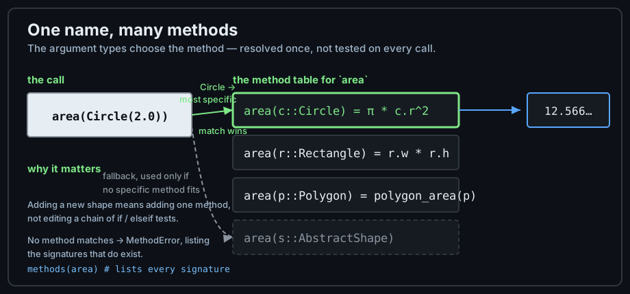
Each signature is a row in the method table. The compiler picks the most specific match, so the "which kind is this?" test is resolved once instead of on every call.

struct Circle;    r::Float64;             end
struct Rectangle; w::Float64; h::Float64; end

area(c::Circle)    = π * c.r^2
area(r::Rectangle) = r.w * r.h

area(Circle(2.0))            # 12.566370614359172
area(Rectangle(2.0, 3.0))    # 6.0
area("not a shape")          # MethodError — no method matches a String

# The function is the collection of its methods:
methods(area)                # 2 methods for generic function "area"

# Methods can be added later, or from another module, without touching the first
struct Triangle; b::Float64; h::Float64; end
area(t::Triangle) = t.b * t.h / 2
area(Triangle(4.0, 3.0))     # 6.0

Type Annotations in Signatures

An annotation on a parameter does two jobs: it constrains which calls are accepted, and it lets the compiler specialise the body. Annotating with an abstract type — AbstractVector, Real, AbstractString — keeps the method usable for every subtype while still documenting the intent.

# Unannotated: accepts anything and cannot help the compiler much
norm1(v) = sum(abs, v)

# Annotated with an abstract type: any AbstractVector works
norm1(v::AbstractVector) = sum(abs, v)
norm1([1, -2, 3])            # 6
norm1(1:3)                   # 6  — a range is an AbstractVector subtype

# Concrete annotations restrict tightly — useful, but think twice
add_ints(a::Int, b::Int) = a + b
add_ints(1, 2)               # 3
add_ints(1.0, 2)             # MethodError: no method matching add_ints(::Float64, ::Int64)

# Annotations select a method — they do not convert the argument
add_ints(Int8(1), Int8(2))   # MethodError: Int8 is not Int, though both are integers

# Annotate with an abstract type when you want the whole family:
add_any_ints(a::Integer, b::Integer) = a + b
add_any_ints(Int8(1), Int8(2))   # 3 — any Integer subtype matches
add_any_ints(1, 2)               # 3

Ambiguity and Specificity

When several methods match, Julia picks the most specific one: a concrete type beats an abstract type, and a method that fits more arguments tightly wins. If two methods are equally specific, the call is ambiguous and raises rather than guessing — an error you will occasionally see from the standard library, and one that always has an explicit fix.

describe(x::Number)  = "a number"
describe(x::Integer) = "an integer"
describe(x::Int)     = "an Int"

describe(3)          # "an Int"    — most specific of the three
describe(Int8(3))    # "an integer" — Int8 is an Integer but not an Int
describe(3.5)        # "a number"
describe("x")        # MethodError — no method for AbstractString

# Ambiguity: neither method is more specific for these arguments
amb(a::Integer, b::Number)  = "A"
amb(a::Number,  b::Integer) = "B"
amb(1, 2)            # MethodError: ambiguous — both are Integer
amb(1, 2.0)          # "A" — Integer+Number is strictly more specific
amb(1.0, 2)          # "B"

Generic versus Concrete

The practical guidance is counter-intuitive at first: leave parameters unannotated unless you need the constraint. An unannotated parameter accepts everything and the compiler still specialises the method for whatever it receives, so no speed is lost — while an over-tight annotation silently excludes types that would have worked.

# ✅ Generic: works for vectors, ranges, tuples, and anything summable
total2(xs) = sum(xs)
total2([1, 2, 3])        # 6
total2(1:3)              # 6
total2((1, 2, 3))        # 6

# ❌ Over-annotated: needs a method for each container you might pass
total3(xs::Vector{Int}) = sum(xs)
total3(1:3)              # MethodError — a range is not a Vector

# Annotate when the constraint IS the point of the function:
#   coefficient_of_rest(r::AbstractFloat) — a formula that only makes sense in floats
#   push_unique!(v::AbstractVector, x)    — the body calls vector-only operations

Functions as Values

Functions are ordinary values: you can bind them to names, store them in collections, return them from other functions, and pass them as arguments. That is what makes map, filter, and sort possible, and it is why Julia code contains far fewer loops than C-like code.

Anonymous Functions

An anonymous function has no name and is written with the arrow syntax x -> expression. It is the standard way to pass a one-off transformation. When the body needs several statements, use the function form inline or define a named function instead.

double = x -> 2x
double(21)                  # 42

# With several arguments
add = (a, b) -> a + b
add(2, 3)                   # 5

# The idiomatic use: a small transformation passed straight in
map(x -> x^2, [1, 2, 3])                      # [1, 4, 9]
filter(x -> x % 3 == 0, 1:20)                 # [3, 6, 9, 12, 15, 18]
sort(["banana", "fig", "plum"]; by = length)  # ["fig", "plum", "banana"]
sort([3, 1, 2]; by = x -> -x)                 # [3, 2, 1] — sort by negated key

# A do block is an anonymous function with the argument at the end
map([1, 2, 3]) do x
    x^2
end                                          # [1, 4, 9]

Composition and Piping

Two operators build new functions out of old ones. f ∘ g composes them (apply g first), and x |> f pipes a value into a call. Both let a multi-step transformation read in the order the data flows, without inventing intermediate names.

# Composition: rightmost function runs first
h = sqrt ∘ abs
h(-16)                 # 4.0 — abs then sqrt

# Composing several
f = round ∘ sqrt ∘ abs
f(-17)                 # 4.0

# Piping: the value on the left becomes the last argument on the right
[1, 2, 3, 4, 5, 6] |> sum                       # 21
[1, 2, 3, 4, 5, 6] |> x -> filter(iseven, x)     # [2, 4, 6]

# Composition of anonymous functions works the same way
scale_then_shift = (x -> x * 2) ∘ (x -> x + 1)
scale_then_shift(3)                              # 8 — (3 + 1) * 2

Closures and Captured State

A closure is a function that captures variables from the scope where it was defined. The captured variable is shared with that scope, not copied, so a closure can carry state between calls — the basis of counters, accumulators, and the do blocks you have already met.

# A counter factory: each call to make_counter returns a fresh closure
function make_counter()
    count = 0
    () -> (count += 1)          # captures `count` by reference
end

c1 = make_counter()
c2 = make_counter()             # an independent counter
c1()                            # 1
c1()                            # 2
c2()                            # 1 — untouched by c1's history

# Accumulating across a loop body
function running_total(xs)
    total = 0.0
    [total += x for x in xs]    # the comprehension sees and updates `total`
end
running_total([1.0, 2.0, 3.0])  # [1.0, 3.0, 6.0]

# Closures over loop variables keep their own binding, as Loops showed:
fs = [() -> i for i in 1:3]
[f() for f in fs]               # [1, 2, 3]

Scope, Mutation, and Recursion

Inside a function, every assignment creates a local variable. Nothing leaks out, nothing is shared unless you ask for it, and the arguments are the only channel in. Understanding this one rule removes almost all the confusion about where a value lives.

local and global

Assignment inside a function body is local by default, so the local keyword is rarely needed — it exists mainly to force a local when a global of the same name would otherwise be picked up. global is the opposite request: write to the variable in the enclosing module. A variable that is used before its first assignment in the same scope raises UndefVarError rather than reading an outer value.

a = 1
b = 2

function demo()
    a = 10          # a NEW local `a`; the global is untouched
    global b = 20   # writes the global
    return a
end

demo()              # 10
a                   # 1  — unchanged
b                   # 20 — changed

# Using a name before assigning it in the same scope is an error
function early()
    println(x)      # ERROR: UndefVarError: `x` not defined
    x = 1
end

# `local` forces a local, which is only needed to shadow deliberately
function shadow()
    local length = 99        # shadows Base.length inside this function only
    length
end
shadow()            # 99
length([1, 2, 3])   # 3  — the real function is unaffected elsewhere

The ! Convention

Julia distinguishes two kinds of function by naming convention: a trailing ! means the function mutates at least one of its arguments. The convention is not enforced by the language, but the standard library follows it strictly, so sort and sort! differ in exactly the way you would hope.

v = [3, 1, 2]

sort(v)         # [1, 2, 3] — a new array; v is unchanged
v               # [3, 1, 2]

sort!(v)        # [1, 2, 3] — sorts in place
v               # [1, 2, 3] — now sorted

# The same pairing runs through the standard library
reverse([1, 2, 3])      # [3, 2, 1] — new
reverse!([1, 2, 3])     # [3, 2, 1] — in place
push!(v, 4)             # appends to v and returns v
unique([1, 1, 2])       # [1, 2]     — new
unique!([1, 1, 2])      # [1, 2]     — in place

# Name your own mutating functions with ! so callers know what to expect
function double!(v)
    v .*= 2
    v
end

Recursion

A function may call itself. Julia has no special syntax or optimisation for it — recursion is ordinary function calls, which means it is fast when the types are stable but has no tail-call elimination, so deep recursion can exhaust the stack. Reach for iteration when the depth is unbounded, and for memoisation when the recursive calls overlap.

function factorial(n)
    n <= 1 ? 1 : n * factorial(n - 1)
end
factorial(5)            # 120

# ⚠ No tail-call elimination: this overflows on large input even though
#   the recursive call is in tail position.
function countdown(n)
    n == 0 && return 0
    countdown(n - 1) + 1
end
countdown(100_000)      # works; deeper values eventually raise StackOverflowError

# Naive Fibonacci recomputes the same values exponentially many times
function fib_slow(n)
    n < 2 ? n : fib_slow(n - 1) + fib_slow(n - 2)
end
fib_slow(30)            # 832040 — 30 already takes a moment

# Memoisation: remember each answer, turning exponential work into linear
const MEMO = Dict{Int,BigInt}()
function fib(n)
    haskey(MEMO, n) && return MEMO[n]
    v = n < 2 ? BigInt(n) : fib(n - 1) + fib(n - 2)
    MEMO[n] = v
    v
end
fib(80)                 # 23416728348467685 — instant, and exact

Notice the two details that make the memoised version work: the cache is a Dict{Int,BigInt} with concrete types, and BigInt avoids the silent integer overflow that a 64-bit Int would hit well before fib(80).

Common Pitfalls

Mutating an Argument by Accident

Arguments are passed by reference, so a function that assigns into an array changes the caller's data. That is a feature when intended and named with !, and a bug when it is a side effect nobody asked for. Copy when the caller's data must survive, and use the non-mutating function when one exists.

function add_one_to_all!(v)
    v .+= 1                  # mutates the caller's array
end

data = [1, 2, 3]
add_one_to_all!(data)
data                         # [2, 3, 4] — intended, and signalled by the !

# If the caller must keep the original, copy first — either at the call
# site or inside the function:
function add_one_safely(v)
    w = copy(v)              # or v[:] for a shallow copy of a vector
    w .+= 1
    w                        # a new array; the argument is untouched
end
kept = [1, 2, 3]
add_one_safely(kept)         # [2, 3, 4]
kept                         # [1, 2, 3] — unchanged

# Scalars are a different matter: numbers are immutable, so reassigning a
# parameter never affects the caller.
function bump(x)
    x += 1                   # a new local binding, nothing else
    x
end
n = 5
bump(n)                      # 6
n                            # 5

Shadowing an Argument

Reassigning a parameter inside the body is legal and sometimes convenient, but it makes the original value unavailable for debugging and can hide a mistake — such as writing x = where x *= was meant. When a function needs a modified version of an argument, give it a new name.

# ❌ The parameter is overwritten: the input is gone from the body onwards
function area_bad(w, h)
    w = w * 2                # is this intended? The reader cannot tell
    w * h
end

# ✅ A new name documents the transformation
function area_good(w, h)
    doubled_w = w * 2
    doubled_w * h
end
area_good(2, 3)              # 12

# The classic typo that shadowing hides:
function discount(price, pct)
    price = price * pct      # overwrote the parameter instead of a temp
    price
end
discount(100, 0.9)           # 90.0 — works, but nothing can inspect the input

Function Barriers

When data is unavoidably untyped — a Vector{Any} read from JSON, for example — the compiler cannot specialise the code that touches it. The remedy is a function barrier: keep the untyped loop minimal and do the real work inside a function, which the compiler can specialise because its arguments have concrete types by then.

# The inner body works on ONE element, so it compiles to tight code
inner(x) = begin
    s = 0.0
    for k in 1:200
        s += x / (k + 1)
    end
    s
end

# ✅ Barrier: the dynamic lookups happen once per element, outside the hot code
function barrier(v)
    t = 0.0
    for x in v
        t += inner(x)        # inner is compiled for the concrete type of x
    end
    t
end

# ❌ Everything inlined: the long inner loop is re-interpreted for every element
function inlined(v)
    t = 0.0
    for x in v
        s = 0.0
        for k in 1:200
            s += x / (k + 1)
        end
        t += s
    end
    t
end

# Measured over a Vector{Any} of 20 000 elements, the barrier version ran
# about 39× faster — the same arithmetic, reached through a typed function.

With dispatch, argument handling, and barriers in hand, the remaining gap in your vocabulary is data: how to store many values, choose the right container, and iterate it efficiently. That is the subject of Collections.