
Expressions & Operators
if, a loop, even an assignment. Operators are then just functions wearing familiar syntax, which is why you can broadcast them across an array or pass + itself to another function.
This lesson builds from the ground up. It starts with the expression model, then covers arithmetic (and the integer-division trap that catches Python programmers), comparisons and their chaining, logic and short-circuit evaluation, bit manipulation, and finally broadcasting — the feature that turns a .+ b into a loop for you, and the single biggest reason Julia code looks unlike C.
Everything Is an Expression
An expression produces a value; a statement performs an action. In C, Java, or Python these are different categories: if is a statement, the ternary ?: is an expression, and you cannot bind an if to a name. Julia has no such split. Blocks, conditionals, loops, and even type definitions are expressions, each evaluating to a value.
The Value of a Block
A begin ... end block evaluates to its last expression, and so does a function body. This is the mechanism behind Julia's concise function syntax, and behind the fact that a function with no explicit return still hands back the final computed value.
# A block is worth its final expression.
x = begin
    1 + 1
    2 + 2
    3 + 3        # ← so the block is worth 6
end
x                # 6

# An `if` is an expression: the value of the chosen branch is the result.
grade = if x > 5
    "pass"
else
    "fail"
end
grade            # "pass"
Assignment Is an Expression
Assignment evaluates to the value assigned, so assignments nest and chain. That is legal and occasionally elegant, but production code keeps one assignment per line — chaining hides where a value was born.
a = b = c = 1     # all three are 1; each assignment is worth 1
(a = 2) + 1       # 3 — the assignment produced 2

# Because `if` returns a value, this reads well:
cached = haskey(dict, key) ? dict[key] : compute(key)
One practical consequence: since the last expression of a function body is its result, a stray trailing expression silently becomes the return value. If a function's final line is println(...), the function returns nothing — usually harmless, occasionally a bug that surfaces three calls later.
Arithmetic Operators
Arithmetic operators are ordinary functions in disguise: a + b parses as +(a, b). That means you can broadcast them, pass them as arguments (map(*, v, 2)), or add methods for your own types. The full set matters mainly for the integer-division family, which is much richer than in C or Python.
Operator Reference
| Expression | Name | Meaning / notes |
|---|---|---|
+x | unary plus | identity — returns x unchanged |
-x | unary minus | additive inverse |
x + y | binary plus | addition |
x - y | binary minus | subtraction |
x * y | times | multiplication; on arrays it is the matrix product |
x / y | divide | true division — always returns a float |
x \ y | inverse divide | equals y / x; reads naturally for matrix solves |
x ^ y | power | exponentiation; 2^-1 gives 0.5 |
div(x, y) | integer division | quotient truncated toward zero |
fld(x, y) | floor division | quotient rounded toward −∞ |
rem(x, y) | remainder | remainder whose sign follows the dividend x |
mod(x, y) | modulo | remainder whose sign follows the divisor y |
x % y | percent | operator form of rem — not modulo |
Integer vs Float Division
The most common arithmetic surprise for newcomers is that / returns a float even when both operands are integers. Julia refuses to truncate silently: integer division must be requested with div or ÷. The second surprise is the rem versus mod split — the two differ exactly when the operands carry different signs.
7 / 2            # 3.5 — Float64, although both operands are Int
7 ÷ 2            # 3   — integer division (÷ is typed \div then Tab)
div(7, 2)        # 3   — truncates toward zero
fld(7, 2)        # 3

div(-7, 2)       # -3  — toward zero
fld(-7, 2)       # -4  — toward minus infinity

# rem takes the dividend's sign; mod takes the divisor's sign.
rem(-7, 2)       # -1  (same sign as -7)
mod(-7, 2)       #  1  (same sign as 2)
-7 % 2           # -1  — % is rem, not mod
Reach for mod when wrapping around a cycle — clock arithmetic, circular buffers, hashing into a fixed number of buckets — because its result always shares the divisor's sign and so never becomes a negative index. Reach for div when splitting items into fixed-size groups, and for fld when you need the mathematically consistent quotient for negative values.
Powers and Precedence
Both ^ and its operator aliases are functions too, and Julia keeps arithmetic precedence close to mathematics: exponentiation binds tighter than multiplication, which binds tighter than addition. The one rule worth memorising is that power is right-associative, so 2^3^2 means 2^(3^2) and not (2^3)^2.
2^3^2            # 512 — right-associative: 2^(3^2) = 2^9
(2^3)^2          # 64  — force the other grouping with parentheses

2^-1             # 0.5 — a negative exponent always yields a float
sqrt(2)          # 1.4142135623730951
√2               # same function; √ is typed \sqrt then Tab
cbrt(27)         # 3.0
abs(-3)          # 3

1 + 2 * 3        # 7 — * before +
(1 + 2) * 3      # 9 — parentheses keep the intent unmistakable
Update Assignment
Every binary arithmetic and bitwise operator has an updating form made by appending =: +=, -=, *=, /=, ^=, %=, ÷=, &=, |=, ⊻=, >>=, <<=. The name is slightly misleading: unlike C, x += 1 is not an in-place memory update. It expands to x = x + 1, so the binding may even change type.
count = 0
count += 1        # count = count + 1 → 1
count *= 10       # count = count * 10 → 10
count ÷= 3        # count = count ÷ 3 → 3

# Because it is a rebinding, the type may change:
x = 1
x /= 2            # x = x / 2 → 0.5; x is now a Float64, not an Int
typeof(x)         # Float64
That last example is a genuine trap: /= quietly turns an integer counter into a float, which then breaks array indexing. When you need true in-place mutation of array contents, use the dotted .+= described in the broadcasting section below.
Comparisons and Chaining
Comparisons produce Bool, and Julia has two features that most languages lack: chained comparisons that read like mathematics, and a four-way family of equality tests that separate value, type, identity, and numeric approximation.
Comparison Operators
| Operator | Name | Notes |
|---|---|---|
== | equality | value equality, may cross numeric types (1 == 1.0) |
!= / ≠ | inequality | negation of == (≠ is \ne + Tab) |
< | less than | ordering; not defined for all types |
<= / ≤ | less than or equal | |
> | greater than | |
>= / ≥ | greater than or equal | |
=== | egal / identity | same object, or equal bits for immutable values |
isequal(x, y) | hash-consistent equality | treats NaN as equal to itself; used by Dict and Set |
≈ | approximate equality | isapprox; ≈ is \approx + Tab |
Chained Comparison
Julia lets you write mathematical chains directly: 0 < x < 10 works as it reads, and — importantly — x is evaluated only once. Python also allows chaining, but C and Java do not: there, 0 < x < 10 compiles to (0 < x) < 10 and is always true because a boolean equals 1. In Julia you write the chain once and it compiles to the correct conjunction.
x = 5
0 < x < 10            # true — exactly what it looks like

# The chain is rewritten as (0 < x) && (x < 10), so x is evaluated once.
calls = Ref(0)
f() = (calls[] += 1; 5)      # a function with an observable side effect
0 < f() < 10                 # true, and calls[] is 1 — f ran once, not twice

# Mixed comparisons chain too:
1 ≤ x ≤ 10            # true for x between 1 and 10 inclusive
"a" <= "b" <= "c"    # true — strings have lexicographic order
Chaining is not only prettier; it avoids repeating a function call. Compare 0 < f(x) < 10 with the manual 0 < f(x) && f(x) < 10, which silently calls f twice and would break outright for a function with side effects.
Equality, Identity, and Approximation
Julia splits what most languages call "equals" into four distinct questions. Choosing the wrong one is a frequent source of subtle bugs, especially because == compares values recursively for collections.
1 == 1.0          # true  — value equality across numeric types
1 === 1.0         # false — different types are not identical

a = [1, 2, 3]
b = [1, 2, 3]
a == b            # true  — same contents
a === b           # false — two distinct arrays in memory
a === a           # true  — the very same object

0.1 + 0.2 == 0.3            # false — floating-point rounding
0.1 + 0.2 ≈ 0.3             # true  — approximate comparison
isapprox(0.1 + 0.2, 0.3)    # true

-0.0 == 0.0        # true  — numerically equal
-0.0 === 0.0       # false — different bit patterns
The rule of thumb: use == for ordinary value comparisons, === when you mean "the same object" or want to distinguish 1 from 1.0, and ≈ for any result that came out of floating-point arithmetic. Use isequal when you need an equality that agrees with hashing — that is what dictionaries use internally, which is why Dict(NaN => 1)[NaN] finds its entry while NaN == NaN is false.
NaN, Missing, and Three-Valued Logic
NaN (not a number) and missing (absent data) both break the assumption that a comparison returns a plain Bool. NaN compares false against everything, including itself; missing propagates through comparisons as missing rather than failing.
NaN == NaN        # false — IEEE 754 semantics
NaN != NaN        # true  — the only value unequal to itself

# Test for NaN with the predicate, never with ==
isnan(NaN)        # true
isnan(1.0)        # false

# missing propagates instead of throwing
missing == 1      # missing
missing > 1       # missing
ismissing(missing)      # true

# Use the three-valued operators for data with missing values
true & missing    # missing
true | missing    # true  — short-circuits to a known answer
coalesce(missing, 0)    # 0 — the second value stands in for missing
Sorting and filtering data that contains missing requires the skipmissing wrapper, which is covered in Collections. The essential habit is that isnan, ismissing, and skipmissing ask the question where == would just return false or missing and hide the problem.
Logic and Short-Circuiting
Boolean logic in Julia uses &&, ||, and !. The two binary operators short-circuit: the right operand may never be evaluated at all. That property is not an optimisation detail — it is a control-flow tool, and it is why idioms like x != 0 && 1/x > 0.5 are safe.
Boolean Operators
| A | B | A && B |
A || B |
!A |
!B |
|---|---|---|---|---|---|
| false | false | false | false | true | true |
| false | true | false | true | true | false |
| true | false | false | true | false | true |
| true | true | true | true | false | false |
Unlike C, Julia has no implicit conversion from integers to booleans. 1 && true is a type error, and if 1 ... end is rejected outright. The only numbers that may stand in for a condition are… none; a condition must be a Bool (or missing, which raises at the point of branching). Use != 0 or !isempty(x) to say what you mean.
true && true      # true
true || false     # true
!true             # false

# No integer-to-Bool coercion — this is a deliberate safety feature.
1 && true        # ERROR: TypeError: non-boolean (Int64) used in boolean context
if 1 end          # ERROR: TypeError

# Say what you mean instead:
if 1 != 0 end     # fine
if !isempty([1]) end
Short-Circuit Evaluation
A && B evaluates B only when A is true; A || B evaluates B only when A is false. Two consequences follow. First, guard clauses become safe. Second, the operators return one of their operands rather than a coerced boolean — a behaviour borrowed from Lisp that makes default-value idioms concise.
# 1. Guard clauses: the division never runs when x is zero.
x = 0
x != 0 && 1 / x > 0.5      # false — and no division happened at all
# (Without the guard this would be Inf > 0.5, which is true, not an error.)

# 2. The result is the deciding operand, not a coerced Bool.
1 < 2 && "yes"             # "yes"
1 > 2 || "fallback"        # "fallback"
a = nothing
b = a === nothing || a     # b is true here — read carefully, see the note below
a === nothing is true, so || short-circuits and returns true — not a. The idiom only works in the other order: a === nothing || return a. When you want a default value, use the ternary, or something when the absent value is nothing — see Control Flow.
The non-short-circuiting forms & and | exist as well: they always evaluate both sides, which is what you want for element-wise operations on arrays and for three-valued logic with missing. Choosing between them is discussed in the next section.
Bitwise Operators
Bitwise operators work on the binary representation of integers and are the fastest operations in the language. They are the right tool for flags, masks, hashing, and low-level protocols — and the wrong tool for logic, because their precedence sits above comparison operators and quietly changes what a condition means.
| Expression | Name | Notes |
|---|---|---|
~x | bitwise not | flips every bit |
x & y | bitwise and | both bits set |
x | y | bitwise or | either bit set |
xor(x, y) / x ⊻ y | bitwise xor | ⊻ is \xor + Tab; the old $ form is deprecated |
x << y | shift left | multiplies by 2y |
x >> y | arithmetic shift right | sign-preserving; divides by 2y |
x >>> y | logical shift right | fills with zeros regardless of sign |
x = 0b1100        # 12 in binary (0b prefix is a binary literal)
y = 0b1010        # 10

x & y             # 0b1000 = 8   (and)
x | y             # 0b1110 = 14  (or)
xor(x, y)         # 0b0110 = 6   (xor)
x ⊻ y             # 0b0110 = 6   (same operator, unicode form)
~x                # -13 — two's complement, so every bit flips

1 << 4            # 16  — shift left is multiply by 2^4
256 >> 4          # 16  — shift right is divide by 2^4
-8 >> 1           # -4  — arithmetic shift keeps the sign
-8 >>> 1          # huge positive number — logical shift fills with zeros
Booleans Are Integers
Bool is a subtype of Integer in Julia, so true is 1 and false is 0 for the purposes of arithmetic and summation. This is deliberate, and it is what makes sum(x > 3 for x in v) a concise way to count matching elements. Note the asymmetry with the section above: a Bool may be used as a number, but a number may not be used as a condition.
true + true       # 2
true * 5          # 5
false - true      # -1
Bool(1)           # true
Int(true)         # 1

# Count how many elements satisfy a predicate — a common idiom.
values = [1, 5, 9, 2, 7]
sum(values .> 3)          # 3 — the comparison mask summed
count(>(3), values)       # 3 — the explicit, clearer form

# Bitwise flags: one bit per option
flags = 0b0001
flags |= 0b0100           # set bit 2 → 0b0101
(flags & 0b0100) != 0     # true — test bit 2 (parenthesised on purpose)
Parenthesising the mask test is not strictly required — in Julia & binds tighter than !=, so the unparenthesised form happens to mean the same thing. In Python it does not, and the equivalent line silently becomes flags & (0b0100 != 0). When you move between the two languages, keep the parentheses and the question never arises.
Broadcasting
Every operator and every function has a broadcasting form, written with a dot: .+, .*, .^, or more generally f.(x). Broadcasting applies the operation element-wise over containers, aligning their shapes and stretching any dimension of length one. It replaces the explicit loop, and because the compiler fuses chained dotted operations into a single pass, it is often both shorter and faster than the loop it replaces.
The Dot Syntax
A dot in front of a function name means "apply this element-wise". In front of an operator the dot fuses with the operator symbol itself. The array is not iterated by a Python-style loop written in the interpreter — the operation is compiled once for the whole call.
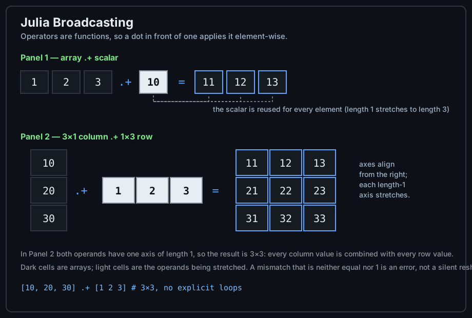
Broadcasting aligns shapes from the right; a length-1 axis stretches to match the other operand. Top: a scalar is reused for every element. Bottom: a column plus a row produces the full 3×3 outer sum.
a = [1, 2, 3]
b = [10, 20, 30]

a .+ b            # [11, 22, 33] — element-wise addition
a .* b            # [10, 40, 90] — element-wise multiplication
a .^ 2            # [1, 4, 9]     — squaring via broadcasting
a .+ 10           # [11, 12, 13]  — a scalar stretches over the whole array

# The plain forms mean linear algebra instead:
a + b             # MethodError — two 1-D arrays cannot be added as vectors
[1 2; 3 4] * [1, 2]   # matrix-vector product, NOT element-wise

# Any function can be broadcast:
sqrt.([1, 4, 9])              # [1.0, 2.0, 3.0]
abs.([-1, 2, -3])             # [1, 2, 3]
join.(string.("x", 1:3), "-") # ["x1-", "x2-", "x3-"]

# Broadcasting over two different shapes aligns from the right:
[10, 20, 30] .+ [1 2 3]       # 3×3 matrix: every pair summed
Fused Broadcasts
Chained dotted operations are merged by the compiler into one loop over the data, so intermediate arrays are never allocated. Fusion is automatic: if every operation in the expression carries the dot, the whole expression is a single broadcast. Introducing one undotted call — even something as ordinary as sum(...) — breaks the chain and materialises a temporary array.
x = rand(1_000_000)

# ✅ Fused: one pass over x, no intermediate arrays.
y = @. x^2 + 3x + 1          # @. adds a dot to every operator in the line

# Equivalent, written out by hand:
y = x.^2 .+ 3 .* x .+ 1

# ❌ Two passes and one temporary vector from the middle expression.
y = x.^2 .+ sum(3 .* x) .+ 1

# Bracket the whole call to broadcast it:
y = sqrt.(x .^ 2 .+ 1)
@. macro from the standard library rewrites the following expression by inserting dots everywhere it can. It is the shortest way to write a fused computation and the safest way to avoid forgetting one dot — a missing dot in a long expression is the most common broadcasting mistake.
In-Place and Assignment Forms
The dotted assignment operators .+=, .-=, .*= and friends are the true in-place operations that the plain += is not: they overwrite the elements of the existing array rather than rebinding the name to a new one. That distinction matters whenever another part of the program holds a reference to the same array.
a = [1.0, 2.0, 3.0]
b = a               # b and a refer to the SAME array

b .+= 10            # in-place: elements of the shared array are updated
a                   # [11.0, 12.0, 13.0] — a sees the change

c = [1.0, 2.0, 3.0]
d = c
d += [10.0, 10.0, 10.0]   # rebinding: creates a new array
c                   # [1.0, 2.0, 3.0] — unchanged
d                   # [11.0, 12.0, 13.0] — a different array

# .+= also avoids allocating, which matters inside a hot loop:
f!(v) = (v .*= 2; v)      # the ! convention signals in-place mutation
Precedence and Readability
Precedence decides which operator grabs its operands first. Julia's order is close to mathematics and close to C, with two deliberate improvements: comparisons chain instead of nesting, and &/| bind tighter than comparisons, so mask tests mean what they say. You almost never need the full table — but you do need to recognise the two or three places where the compiler's grouping is not the one you assumed.
Precedence Table
| Level | Operators | Associativity |
|---|---|---|
| 1 — syntax | . :: | left |
| 2 — exponent | ^ | right |
| 3 — unary | + - √ ! ~ | prefix (right) |
| 4 — bitshift | << >> >>> | left |
| 5 — multiplicative | * / % & \ ÷ | left |
| 6 — additive | + - | ⊻ | left |
| 7 — comparison | < <= > >= == != === !== ≈ | chainable |
| 8 — logical and | && | left, short-circuits |
| 9 — logical or | || | left, short-circuits |
| 10 — ternary | ? : | right |
| 11 — assignment | = += -= .+= … | right |
# Level 2 beats level 5: exponentiation first.
2 * 3^2               # 18, not 36

# Unary minus is level 3 and ^ is level 2, so ^ wins the operand.
-2^2                  # -4  (i.e. -(2^2)), unlike some calculators
(-2)^2                # 4   — parenthesise when you mean this

# Levels 5 and 6: & binds tighter than +, which surprises C programmers.
1 + 2 & 3             # 3 — parsed as 1 + (2 & 3), not (1 + 2) & 3

# Level 7 is chainable; levels 8-10 are not, so the ternary needs no parens here.
x = 5
0 < x < 10            # true
x > 0 ? "pos" : "neg" # "pos"
Symbols and Punctuation
Julia reuses a small set of symbols for several purposes, and a few of them are conventions rather than operators. The table below collects the ones you will meet in ordinary code.
| Symbol | Meaning |
|---|---|
@m | invoke macro m; followed by space-separated expressions |
! prefix | logical negation operator |
f!() | naming convention: the function mutates its argument(s) |
' | adjoint (conjugate transpose) — A' |
::T | type assertion on a value, or type constraint on a field/parameter |
:sym | Symbol literal — an interned name, not a string |
-> | anonymous function: x -> x^2 |
$ | interpolation inside strings and quoted expressions |
... | splat / slurp in argument lists |
=> | Pair constructor — used by dictionaries and named tuples |
; | separates statements on one line; inside brackets it separates array rows or keyword arguments |
# / #= =# | line comment / nestable block comment |
Common Pitfalls
Forgetting the Dot — or Adding It
The dot is not decoration: * is a matrix product while .* is element-wise, and ^ on a matrix means repeated matrix multiplication while .^ squares each entry. Mixing them up produces either a DimensionMismatch or — worse — a numerically plausible wrong answer.
A = [1 2; 3 4]

A * A             # [7 10; 15 22]  — true matrix product
A .* A            # [1 4; 9 16]    — element-wise squares
A^2               # [7 10; 15 22]  — same as A * A
A .^ 2            # [1 4; 9 16]    — element-wise, no linear algebra

# Scalar-exponent vs element-wise exponent, again:
A^0.5             # ERROR or matrix square root — never what a beginner wants
A .^ 0.5          # element-wise square root — almost always the intent
Mixing && with Bitwise Operators
&& and & are different operators with different guarantees: only the first short-circuits. Writing & where you meant && is not a syntax error — it compiles and runs, and simply evaluates the right-hand side even when the left already decided the answer. In a loop that right-hand side might be an expensive call or one that assumes a precondition.
v = Int[]
len = length(v)

# ❌ Both sides evaluate: indexing an empty array raises BoundsError.
len > 0 & v[1] > 0        # ERROR

# ✅ Short-circuit: the second test never runs when len is 0.
len > 0 && v[1] > 0      # false, no error

# The same rule inside a condition:
if len > 0 && v[1] > 0
    println("first element is positive")
end
Comparing Floats with ==
Floating-point arithmetic is not exact, so == on computed floats is a coin flip. Every quantity that arrives through a division, a square root, or a sum of decimals should be compared with ≈ and an explicit tolerance.
0.1 + 0.2 == 0.3              # false
0.1 + 0.2 ≈ 0.3               # true

# Control the tolerance when the magnitudes are unusual.
isapprox(1e10, 1e10 + 1)                 # true by default relative tolerance
isapprox(1e10, 1e10 + 1; atol = 0)       # false — demand absolute exactness

# Testing exact zero after cancellation is the classic trap.
x = 1e-16
x == 0                        # false, although the value is "zero" for the physics

# The safe pattern
abs(x) < 1e-12               # true — an explicit tolerance you chose yourself
Choose the tolerance deliberately: 1e-12 is reasonable for double precision with order-1 magnitudes, but a relative test with rtol is more robust when values span many orders of magnitude. Whatever you pick, writing it down is the point — an implicit default hides the assumption.
With expressions, comparisons, logic, bit manipulation, and broadcasting in hand, you have the complete vocabulary for computing single values and whole arrays at once. Next: Control Flow turns these expressions into decisions, and then Loops & Iteration repeats them.